Video
Watch the full video
Annotated Presentation
Below is an annotated version of the presentation, with timestamped links to the relevant parts of the video for each slide.
Here is the annotated presentation based on the provided video transcript and slide summaries.
1. The Spark of the AI Revolution
The presentation begins with the title slide, “The Spark of the AI Revolution: Transfer Learning,” presented by Rajiv Shah from Snowflake. This talk was originally given at the University of Cincinnati and recorded later to share the insights with a broader audience.
Rajiv sets the stage by explaining that this is not a deep technical dive into code, but rather a descriptive history and analysis of the drivers behind the current AI boom. The goal is to explain how AI learns and how individuals can start to interrogate and understand these technologies in their own lives.
The core premise is that Transfer Learning is the catalyst that shifted AI from academic curiosity to a revolutionary force. The talk aims to bridge the gap for those unfamiliar with the underlying mechanics of how models like ChatGPT came to be.
2. Sparks of AGI: Early Experiments
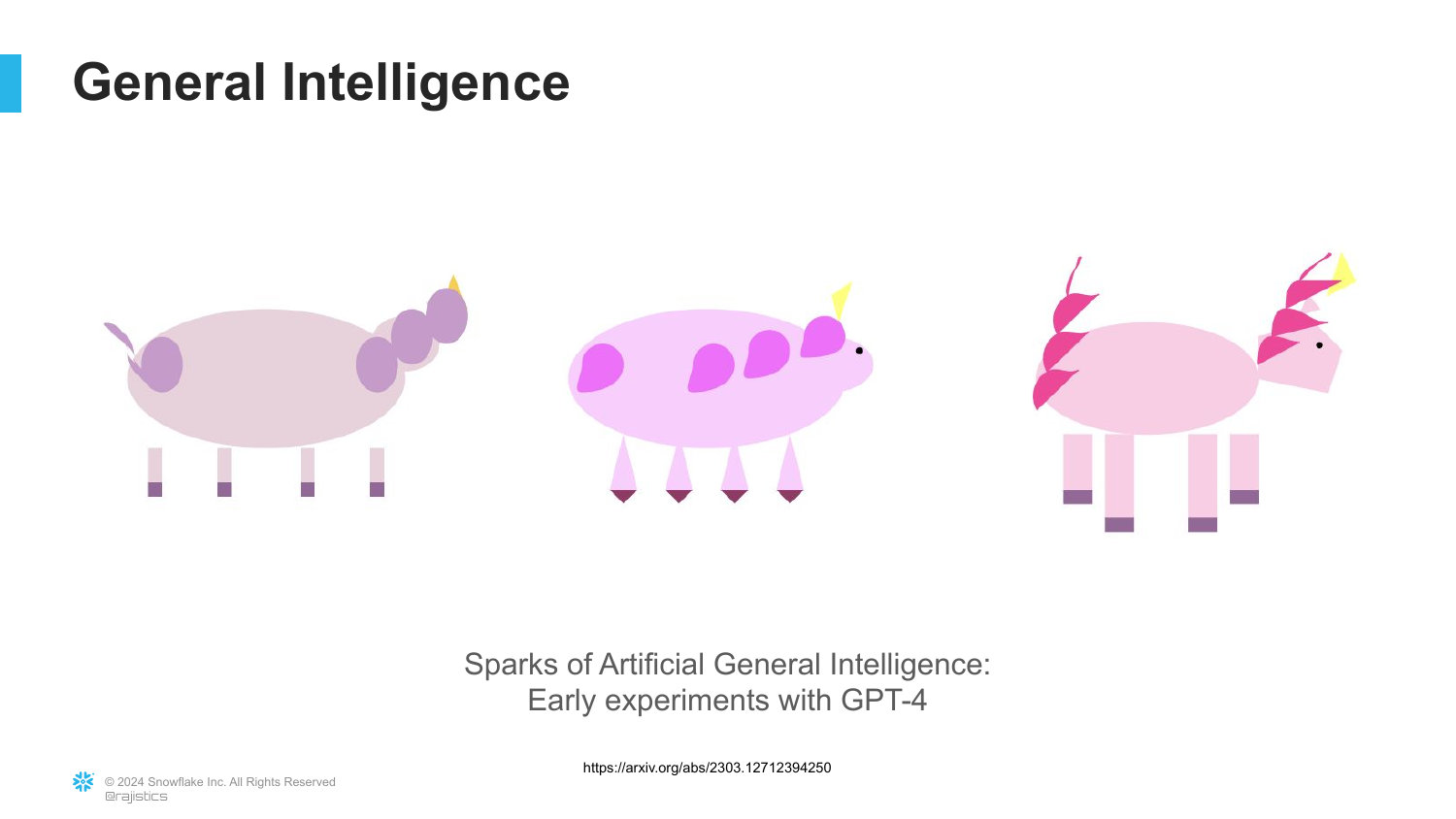
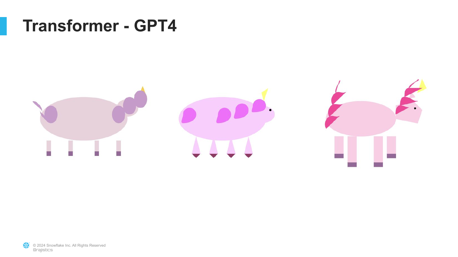
This slide illustrates an early experiment conducted by researchers investigating GPT-4. To understand how the model was learning, they gave it a concept and asked it to draw it using code (SVG). The slide displays a progression of abstract animal figures, showing how the model’s ability to represent concepts improved over time during training.
This references the paper “Sparks of Artificial General Intelligence,” which caused significant waves in the tech community. It suggests that these models were beginning to show signs of Artificial General Intelligence (AGI)—reasoning capabilities that extend beyond narrow tasks.
The visual progression from crude shapes to recognizable forms serves as a metaphor for the rapid evolution of these models. It highlights the mystery and potential power hidden within the training process of Large Language Models (LLMs).
3. Extinction Level Threat?
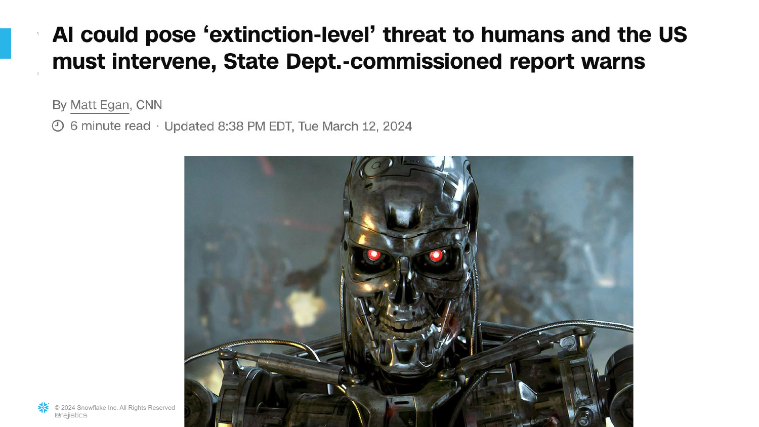
The presentation addresses the extreme concerns surrounding the rapid scaling of AI technologies. The slide features a dramatic image reminiscent of the Terminator, referencing fears that unchecked AI development could pose an “extinction-level” threat to humanity.
Rajiv notes that as these technologies scale, there is a segment of the research and safety community worried about catastrophic outcomes. This sets up a contrast between the theoretical existential risks and the practical, everyday reality of how AI is currently being used.
This slide acknowledges the “hype and fear” cycle that dominates the media narrative, validating the audience’s anxiety before pivoting to a more grounded explanation of how the technology actually works.
4. The New AI Overlords
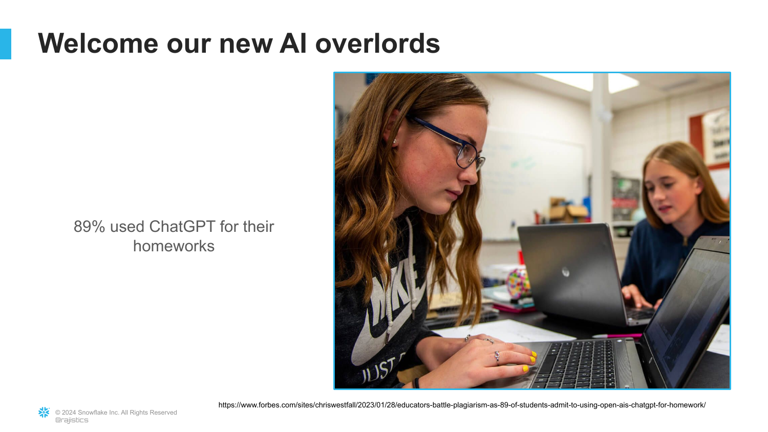
Shifting to a lighter tone, this slide highlights the widespread adoption of AI by the younger generation. It cites a statistic that 89% of students have used ChatGPT for homework, humorously suggesting that children have already “accepted our new AI overlords.”
The slide points out a discrepancy in honesty, noting that while 89% use it, a significant portion (implied by the “11% are lying” joke) might not admit it. This reflects a fundamental shift in education and information retrieval that has already taken place.
This context emphasizes that the AI revolution is not just a future possibility but a current reality affecting how the next generation learns and works. It underscores the urgency of understanding these tools.
5. Fundamental Questions

This slide poses the central questions that the presentation will answer: “What is AI doing?” and “How should you think about AI?” It serves as an agenda setting for the technical explanation that follows.
Rajiv transitions here from the societal impact of AI to the mechanics of machine learning. He prepares the audience to look “under the hood” to demystify the “magic” of tools like ChatGPT.
The goal is to move the audience from passive consumers of AI hype to critical thinkers who understand the limitations and capabilities of the technology based on how it is built.
6. How We Teach Computers
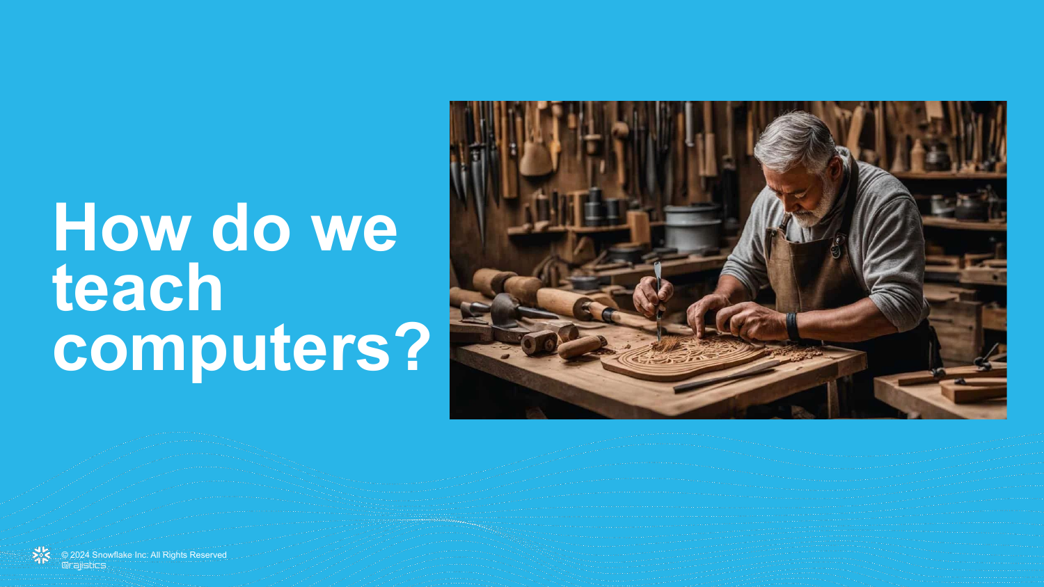
The presentation begins its technical explanation with a fundamental question: “How do we teach computers?” The slide uses imagery of blueprints and tools, likening the traditional process of building AI models to craftsmanship.
This introduces the concept of Supervised Learning in a relatable way. Before discussing neural networks, Rajiv grounds the audience in traditional analytics, where humans explicitly guide the machine on what to look for.
The focus here is on the human element in traditional machine learning—the “artisan” who must carefully select inputs to get a desired output.
7. Identifying Features
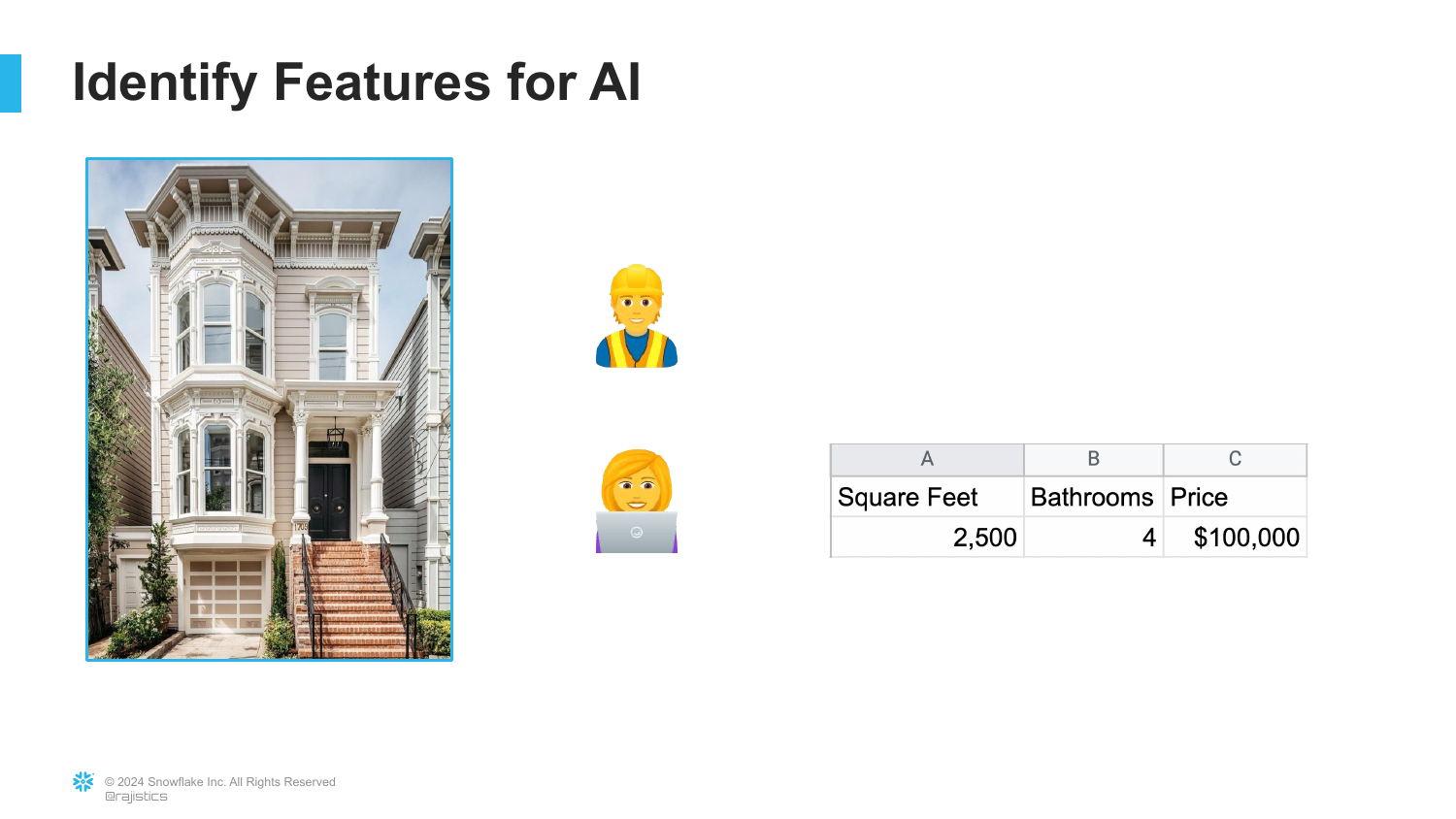
Using a real estate example, this slide explains the concept of Features (or variables). To teach a computer to value a house, one must identify specific characteristics like square footage, number of bedrooms, or closet space.
Rajiv explains that we capture these characteristics and organize them into a tabular format. This process is known as Feature Engineering, where the data scientist decides which attributes are relevant for the problem at hand.
This is the bedrock of traditional enterprise AI: converting real-world objects into structured data points that a machine can process mathematically.
8. Historical Data Patterns
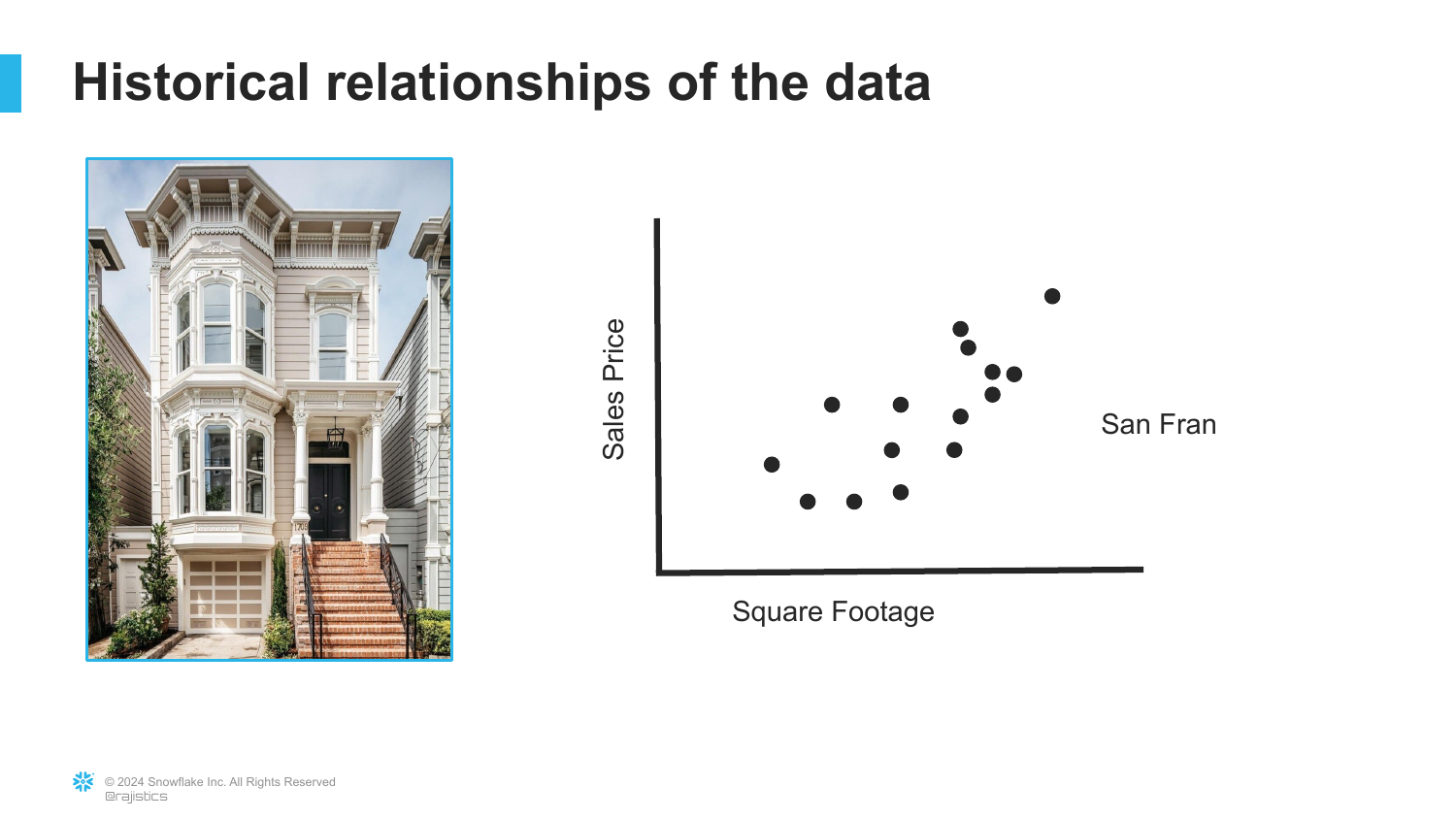
This slide displays a scatter plot correlating “Sales Price” with “Square Feet.” It illustrates how enterprises gather historical data to look for patterns and relationships backwards in time.
Rajiv notes that much of traditional analytics is simply looking at this historical data to understand what happened. However, the power of AI lies in using this data for forward-looking purposes.
The visual clearly shows a trend: as square footage increases, the price generally increases. This linear relationship is what the machine needs to “learn.”
9. Learning the Model
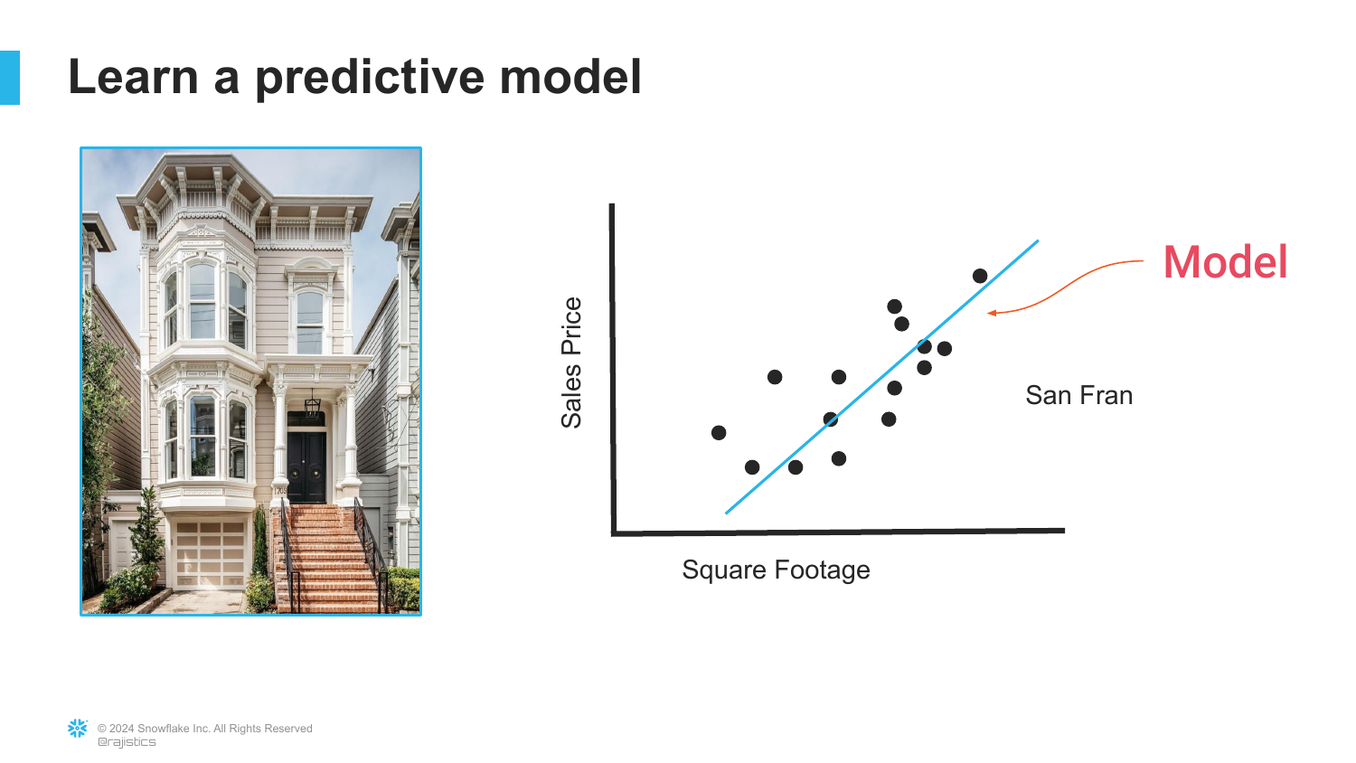
Here, a line is drawn through the data points on the scatter plot. This line represents the Model. Learning, in this context, is simply the mathematical process of fitting this line to the historical data to minimize error.
Rajiv explains that the model “understands the relationships” defined by the data. Instead of a human manually writing rules, the algorithm finds the best-fit trend based on the input features.
This simplifies the concept of training a model down to its essence: finding a mathematical representation of a trend within a dataset.
10. Making Predictions
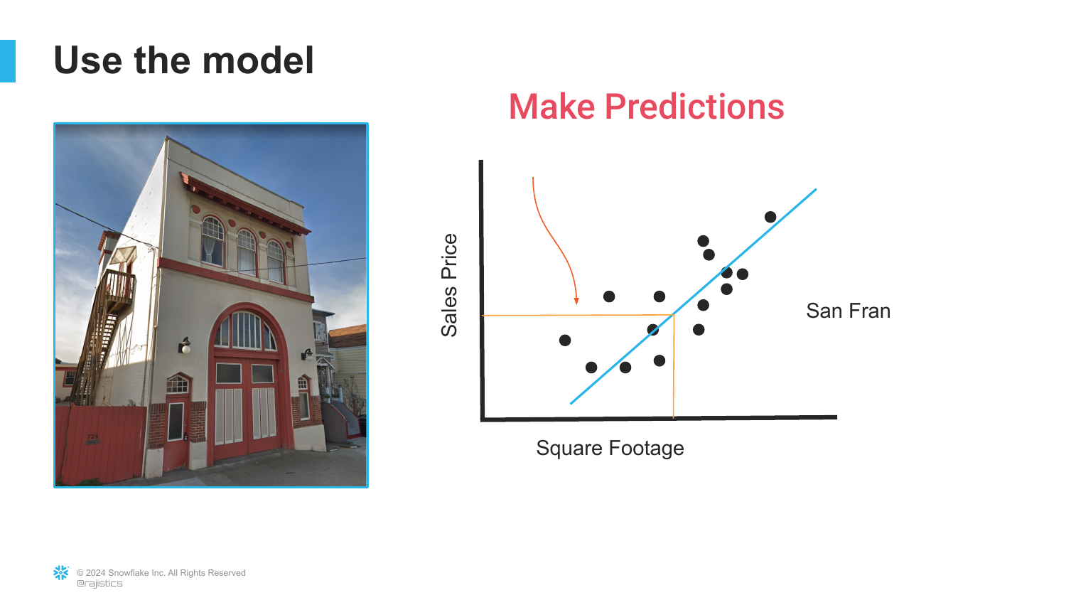
This slide demonstrates the utility of the trained model. When a “New House” comes onto the market, the model uses the learned line to predict its value based on its square footage.
This defines the Inference stage of machine learning. The model is no longer learning; it is applying its “knowledge” (the line) to unseen data to generate a prediction.
It highlights the portability of a model—once trained, it can be used to make rapid assessments of new data points without human intervention.
11. The Domain Limitation
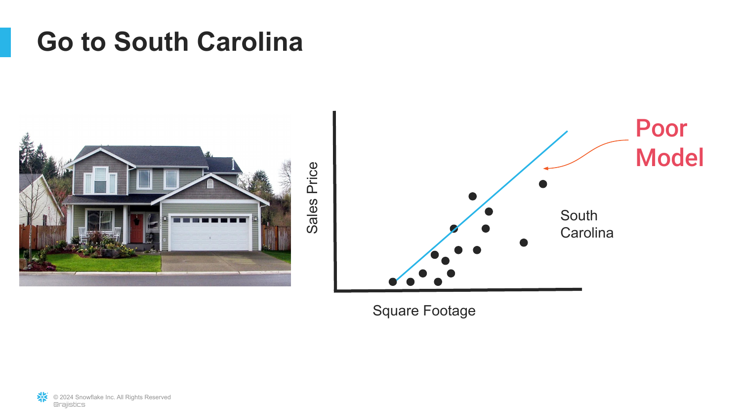
The presentation introduces a critical limitation of traditional models. The slide shows the model trained on San Francisco data being applied to houses in South Carolina. The result is labeled “Poor Model.”
Rajiv explains that while you can technically take the model with you, it will fail because the underlying relationships between features (size) and targets (price) are different in different domains (geographies).
This illustrates the concept of Domain Shift or lack of generalization. A model is only as good as the data it was trained on, and it assumes the future (or new location) looks exactly like the past.
12. The Thinking Emoji
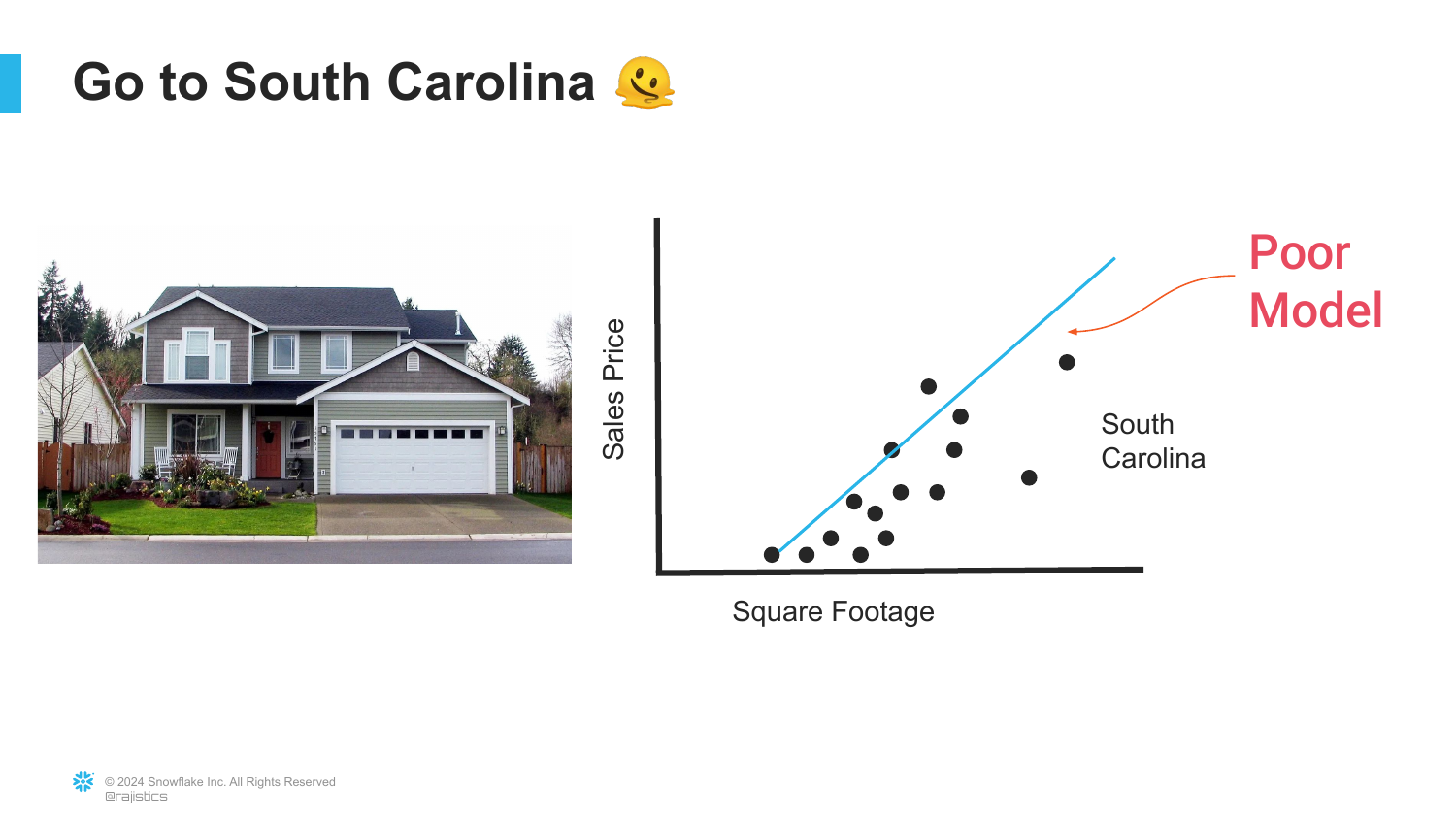
This slide reinforces the previous point with a thinking emoji, emphasizing the realization that the existing model is inadequate. The “San Francisco Model” does not fit the “South Carolina Data.”
It serves as a visual pause to let the problem sink in: traditional machine learning is brittle. It requires the data distribution to remain constant.
Rajiv uses this to set up the labor-intensive nature of traditional analytics, where models cannot simply be “transferred” across different contexts.
13. Train New Model
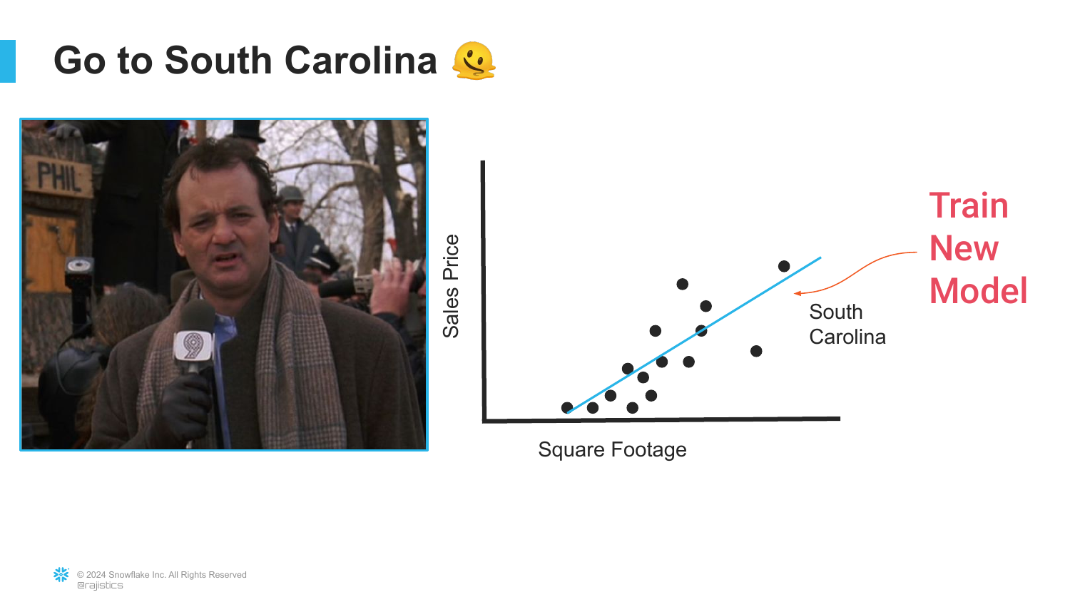
The solution in the traditional paradigm is presented here: “Train New Model.” To get accurate predictions for South Carolina, one must collect local data and repeat the entire training process from scratch.
This highlights the “Never-Ending Battle” of enterprise analytics. Data scientists are constantly retraining models for every specific region, product line, or use case.
This sets the baseline for why Transfer Learning (introduced later) is such a revolution. In the old way, knowledge was not portable; every problem required a bespoke solution.
14. Artisan AI
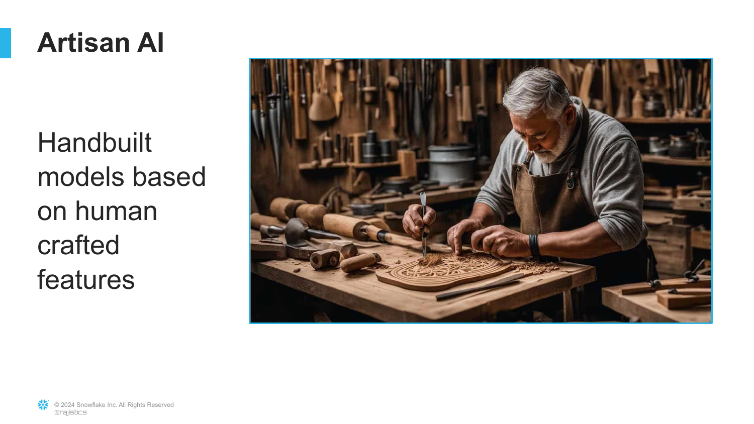
Rajiv coins the term “Artisan AI” to describe this traditional approach. The slide features an image of a craftsman, symbolizing that these models are hand-built and rely heavily on human-crafted features.
This approach is slow and difficult to scale. Just as an artisan can only produce a limited number of goods, a data science team using these methods can only maintain a limited number of models.
It emphasizes that the intelligence in these systems comes largely from the human who engineered the features, not the machine itself.
15. Enterprise AI Use Cases
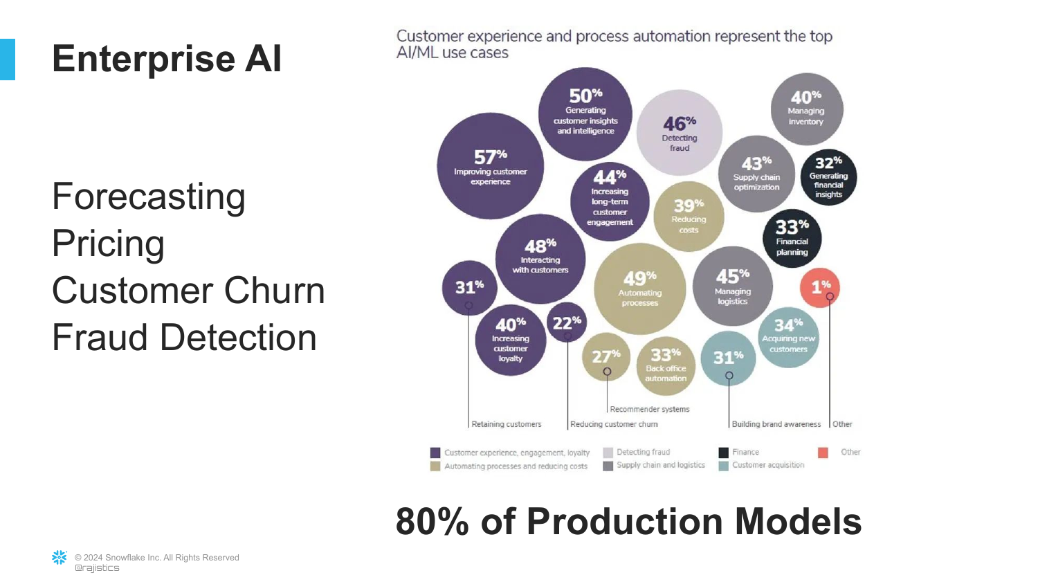
This slide lists common Enterprise AI applications: Forecasting, Pricing, Customer Churn, and Fraud. It notes that 80% of production models currently fall into this category.
Rajiv grounds the talk in the reality of today’s business world. Despite the hype around Generative AI, most companies are still running on these “Artisan” structured data models.
This distinction is crucial for understanding the market. There is “Old AI” (highly effective, structured, labor-intensive) and “New AI” (generative, unstructured, scalable), and they solve different problems.
16. The Computer Science Perspective
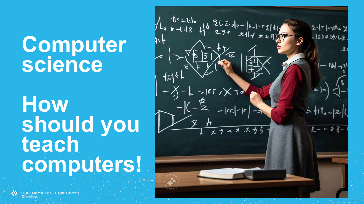
The presentation shifts from the enterprise view to the academic Computer Science view. The slide asks, “How should we teach computers?” signaling a move toward more advanced methodologies.
Rajiv indicates that computer scientists were trying to find ways to move beyond the limitations of manual feature engineering. They wanted machines to learn the features themselves.
This transition introduces the concept of Deep Learning and the move toward processing unstructured data like audio, images, and text.
17. Frederick Jelinek’s Insight
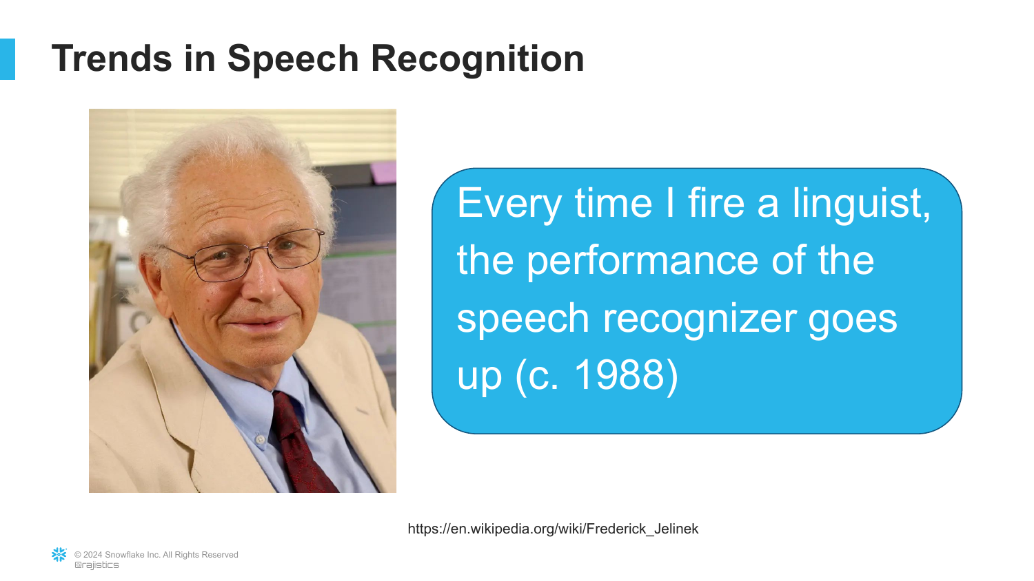
This slide introduces a quote from Frederick Jelinek, a pioneer in speech recognition: “Every time I fire a linguist, the performance of the speech recognizer goes up.”
This provocative quote encapsulates a major shift in AI philosophy. It suggests that human expertise (linguistics) often gets in the way of raw data processing. Instead of hard-coding grammar rules, it is better to let the model learn patterns directly from the data.
Rajiv asks the audience to “chew on that,” as it foreshadows the “Bitter Lesson” of AI: massive compute and data often outperform human domain expertise.
18. Computer Vision in 2010
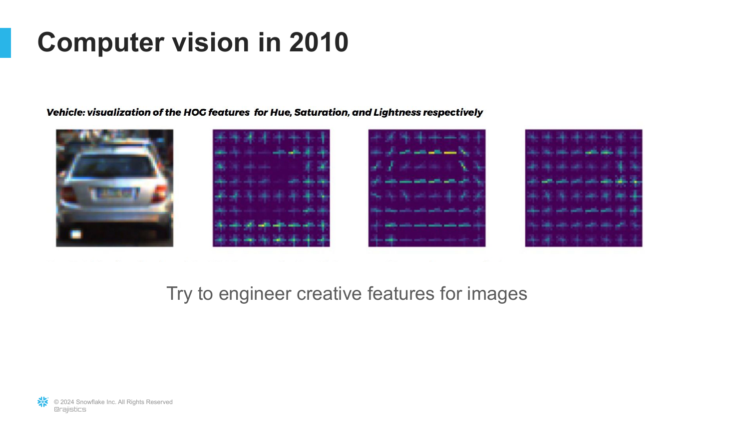
The slide depicts the state of Computer Vision around 2010. It shows a process of manual feature extraction (like HOG - Histogram of Oriented Gradients) used to identify shapes and edges.
Rajiv explains that even in vision, researchers were essentially doing “Artisan AI.” They sat around thinking about how to mathematically describe the shape of a car or a truck to a computer.
This illustrates that before the deep learning boom, computer vision was stuck in the same “feature engineering” trap as tabular analytics.
19. SVM Classification
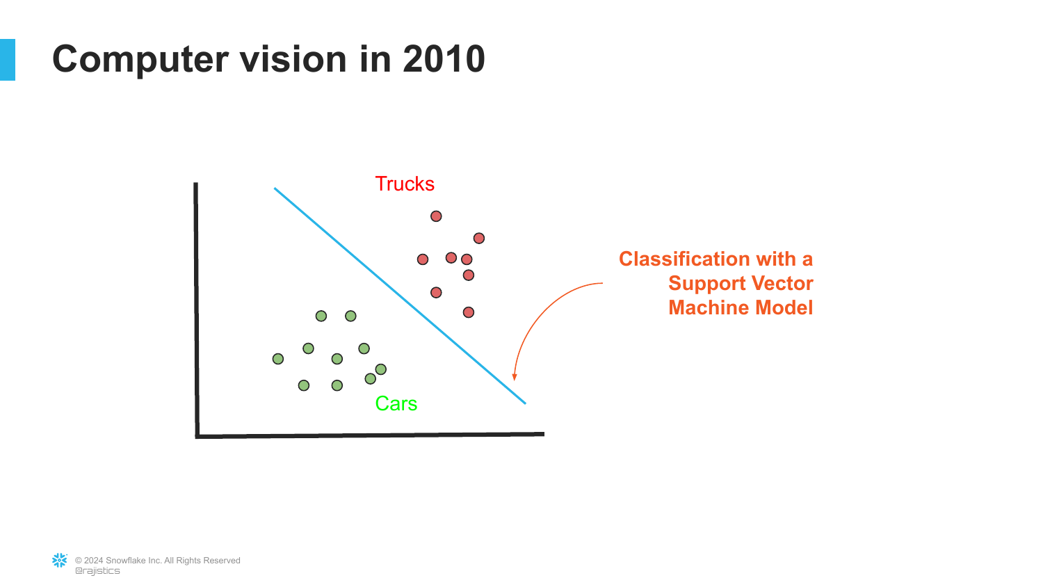
Following feature extraction, this slide shows a Support Vector Machine (SVM) classifier separating data points (cars vs. trucks). This was the standard approach: extract features manually, then use a simple algorithm to classify them.
This reinforces the previous point about the limitations of the time. The intelligence was in the manual extraction, not the classification model.
Rajiv mentions his own work at Caterpillar, noting that this was exactly how they tried to separate images of machinery—a tedious and specific process.
20. Fei-Fei Li and Big Data

The slide introduces Professor Fei-Fei Li, a visionary in computer vision. It features a collage of images, hinting at the need for scale.
Rajiv explains that Fei-Fei Li recognized that for computer vision to advance, it needed to move away from tiny datasets (100-200 images) and toward massive scale. She understood that deep learning required vast amounts of data to generalize.
This marks the beginning of the “Big Data” era in AI, where the focus shifted from better algorithms to better and larger datasets.
21. ImageNet
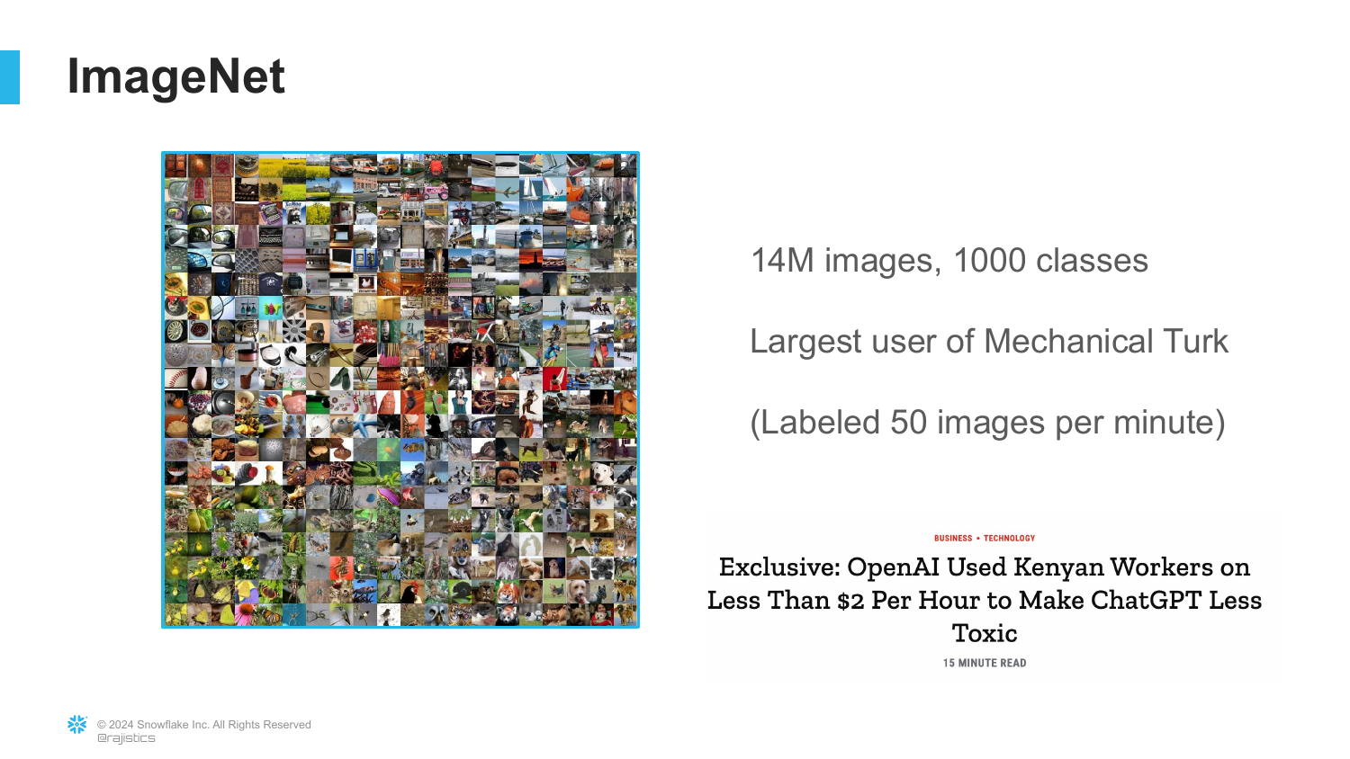
This slide details ImageNet, the dataset Fei-Fei Li helped create. It contains 14 million images across 1000 classes.
Rajiv highlights the sheer effort involved, noting the use of Mechanical Turk to crowdsource the labeling of these images. He calls this the “dirty secret” of AI—that it is powered by low-wage human labor labeling data.
ImageNet became the benchmark that drove the AI revolution. It provided the “fuel” necessary for neural networks to finally work.
22. AlexNet and GPUs

The presentation introduces Alex Krizhevsky, a graduate student under Geoffrey Hinton. The slide mentions “AlexNet” and the use of GPUs (Graphics Processing Units).
Rajiv tells the story of how Alex decided to use NVIDIA gaming cards to train neural networks. Traditional CPUs were too slow for the math required by deep learning.
This moment—combining the massive ImageNet dataset with the parallel processing power of GPUs—was the “big bang” of modern AI.
23. AlexNet Training Details
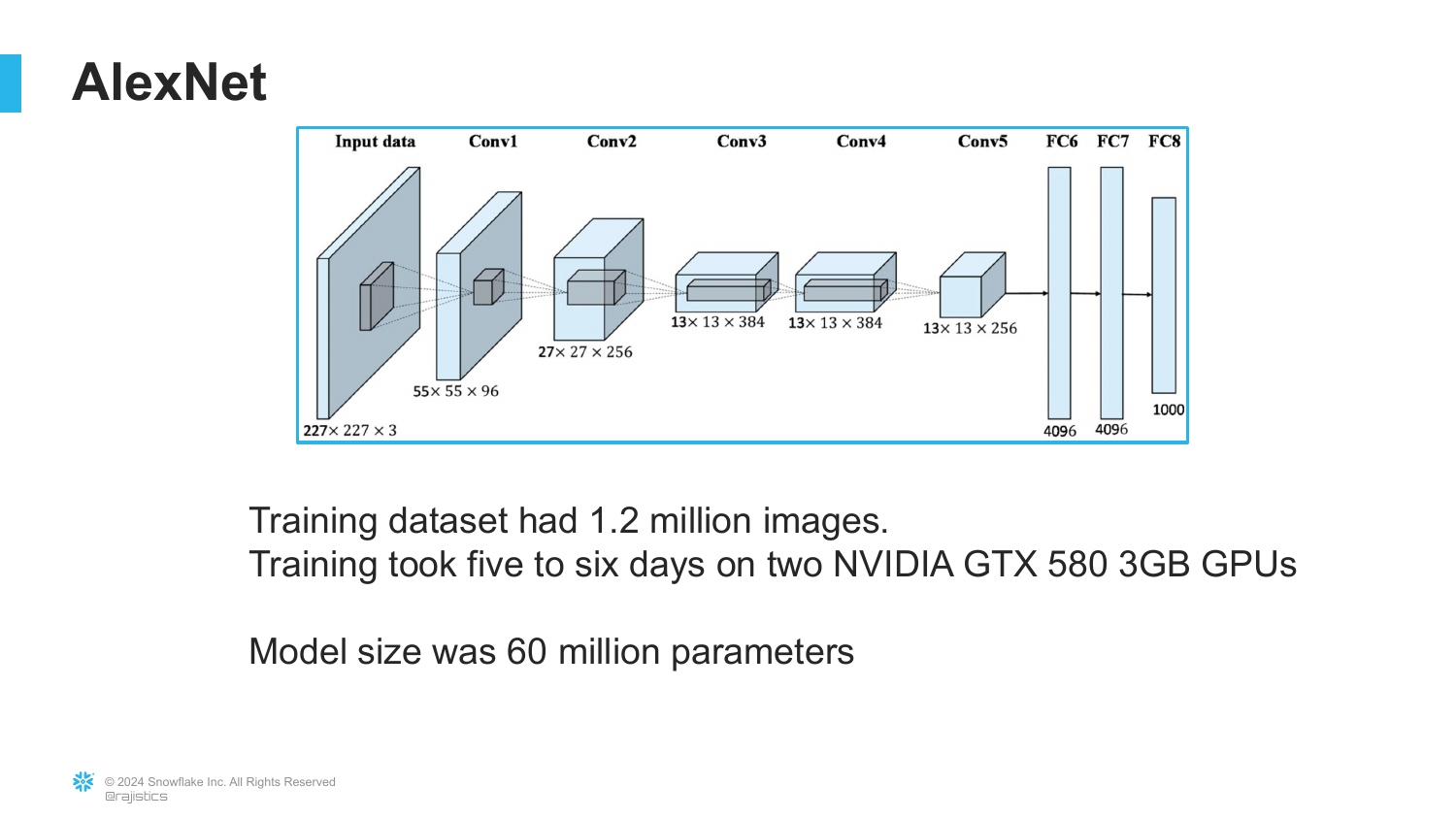
This slide provides the technical specs of AlexNet: trained on 1.2 million images, using 2 GPUs, taking roughly 6 days, with 60 million parameters.
Rajiv emphasizes that while 6 days seems long, the result was a model vastly superior to anything else. It proved that neural networks, which had been theoretical for decades, were now practical.
The “60 million parameters” figure is a precursor to the “billions” and “trillions” we see today, marking the start of the parameter scaling race.
24. Crushing the Competition
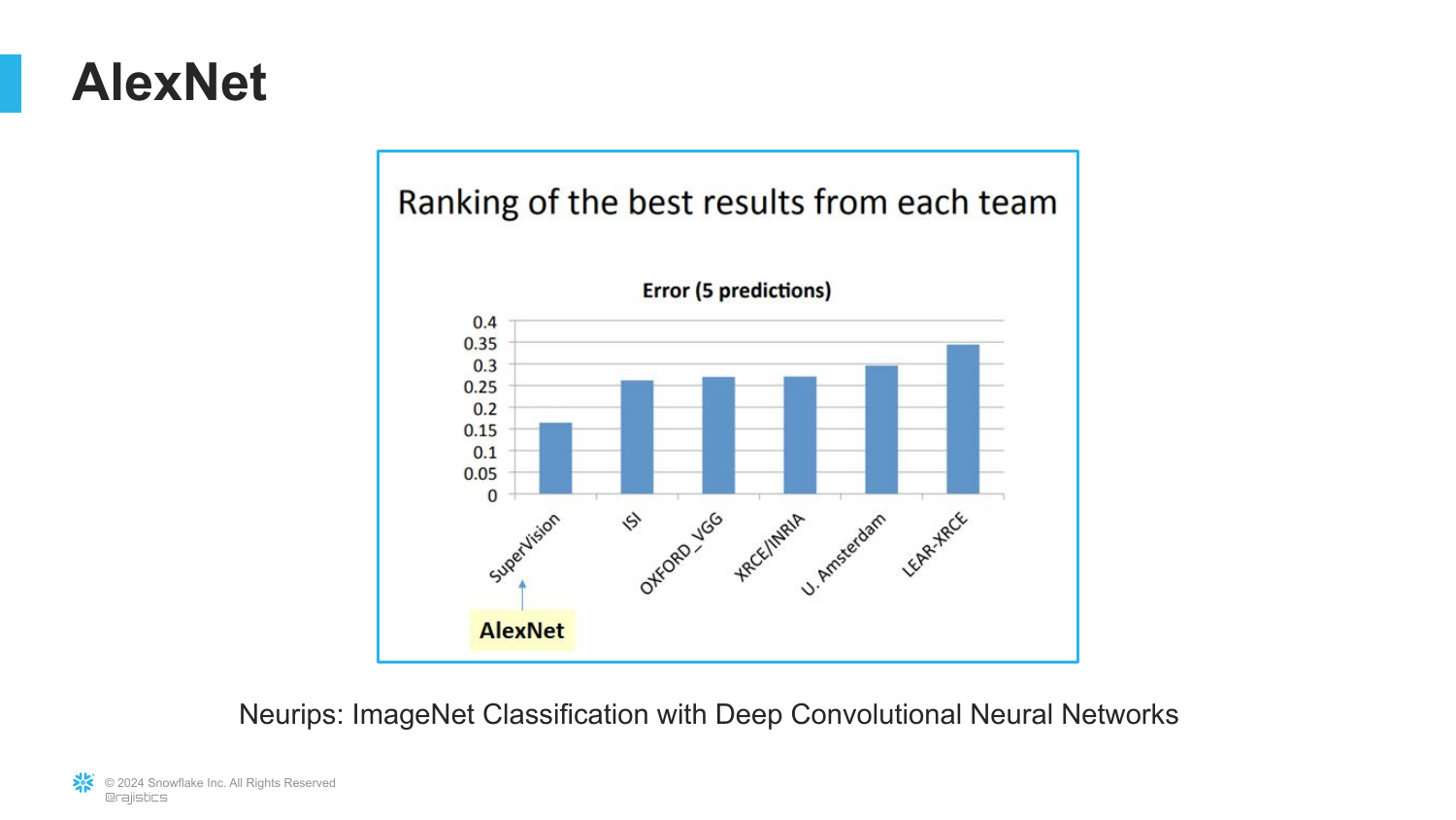
A chart displays the results of the ImageNet Large Scale Visual Recognition Challenge. It shows AlexNet achieving a significantly lower error rate than the competitors.
Rajiv notes that the performance jump was so dramatic that by the following year, every competitor had switched to using the AlexNet architecture.
This visualizes the paradigm shift. The “Artisan” methods were instantly obsolete, replaced by Deep Learning.
25. Feature Engineering vs. Deep Learning
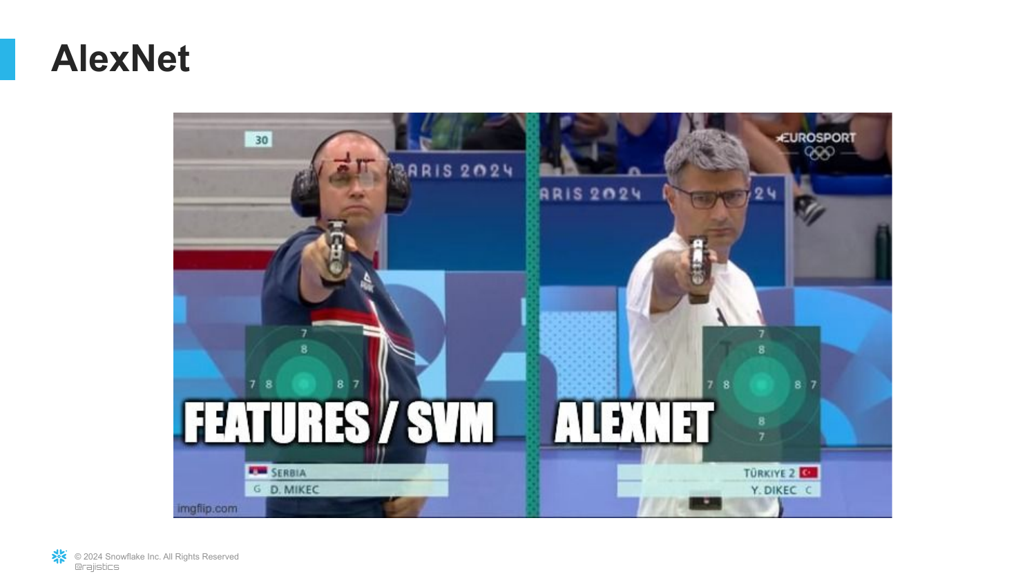
Using a humorous meme format, this slide compares the “Old Way” (Feature Engineering + SVM) with the “New Way” (AlexNet). The AlexNet side is depicted as a powerful, overwhelming force.
This solidifies the takeaway: Deep Learning didn’t just improve upon the old methods; it completely replaced them for unstructured data tasks like vision.
It emphasizes that the model learned the features itself (edges, textures, shapes) rather than having humans manually code them.
26. The 1000 Classes
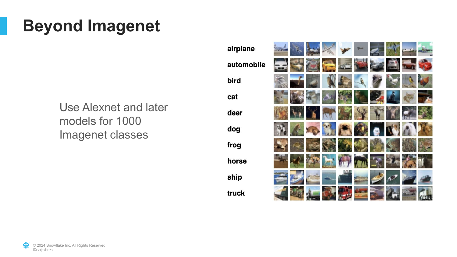
This slide shows examples of the 1000 classes in ImageNet, ranging from specific dog breeds to everyday objects.
Rajiv explains that this model learned to identify a vast array of things from the raw pixels. It went from raw vision to understanding textures, shapes, and objects.
However, he sets up the next problem: What if you want to identify something not in those 1000 classes?
27. The Hot Dog Problem
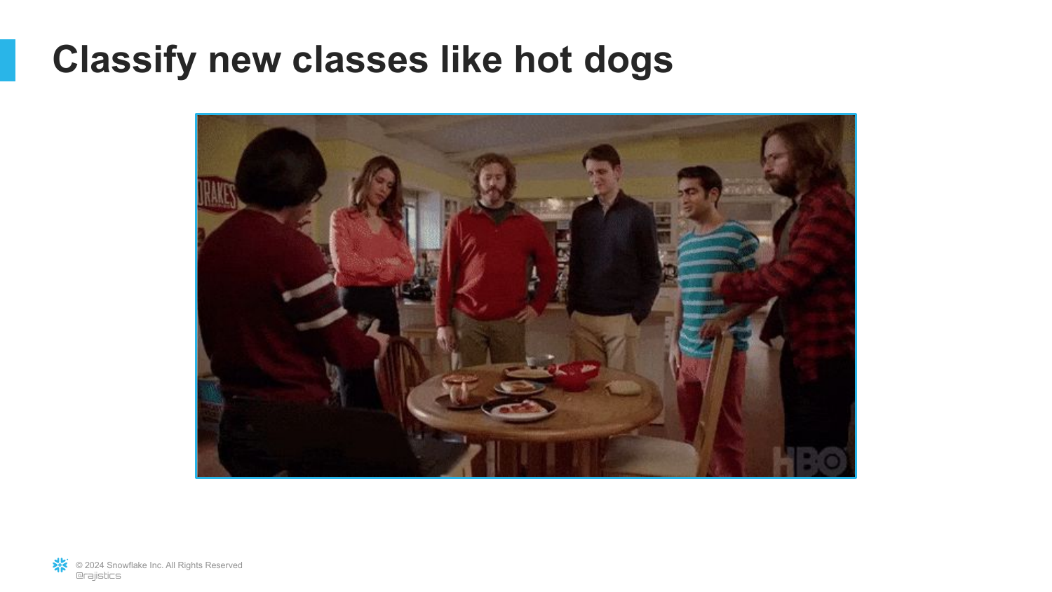
referencing a famous scene from the show Silicon Valley, this slide presents the specific challenge of classifying “Hot Dogs.”
Rajiv uses this to ask: How do you help a buddy with a startup who needs to find hot dogs if “hot dog” isn’t one of the primary categories, or if they need a specific type of hot dog? Do you have to start from scratch?
This sets the stage for Transfer Learning—the solution to avoiding the need for 14 million images every time you have a new problem.
28. Pre-Trained Models

The slide introduces the concept of a Pre-trained Model. This is the model that has already learned the 1000 classes from ImageNet.
Rajiv explains that this model already “knows” how to see. It understands edges, curves, and textures. This knowledge is contained in the “weights” of the neural network.
The key idea is that we don’t need to relearn how to “see” every time we want to identify a new object.
29. Transfer Learning Mechanics

This technical slide illustrates how Transfer Learning works. It shows the layers of a neural network. We keep the early layers (which know shapes and textures) and only retrain the final layers for the new task (e.g., identifying boats).
Rajiv explains that we can transfer “most of that knowledge” and only change a small amount of parameters (less than 10%).
This is the revolution: You can build a world-class model with a small amount of data by standing on the shoulders of the giant ImageNet model.
30. The Revolution
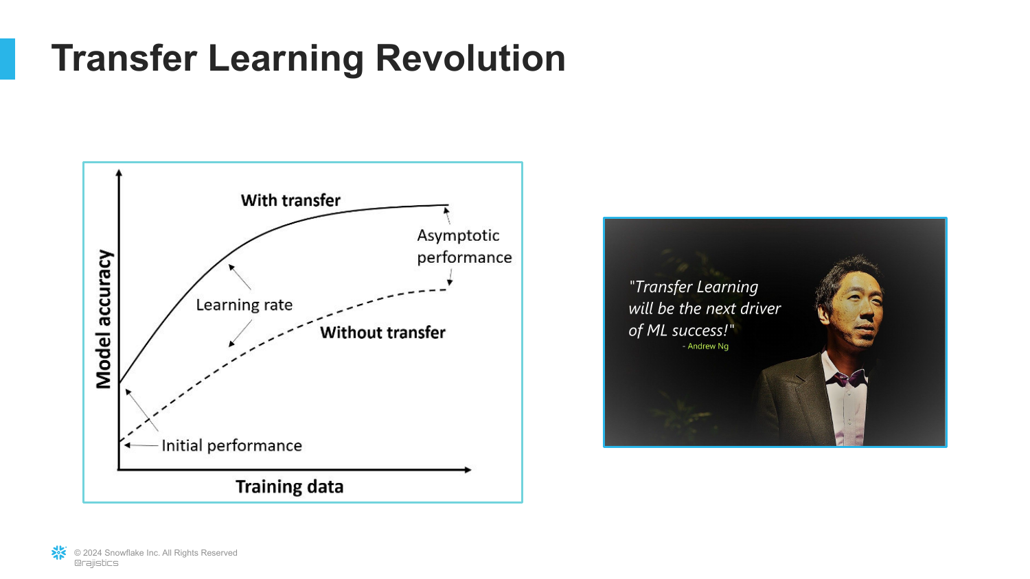
A graph titled “Transfer Learning Revolution” shows the dramatic improvement in accuracy when using transfer learning versus training from scratch. It includes a quote from Andrew Ng stating that transfer learning will be the next driver of commercial success.
Rajiv emphasizes that this capability allowed startups and companies to build powerful AI without needing Google-sized datasets. It democratized access to high-performance computer vision.
This wraps up the vision section of the talk, establishing Transfer Learning as the “Spark.”
31. The Implications
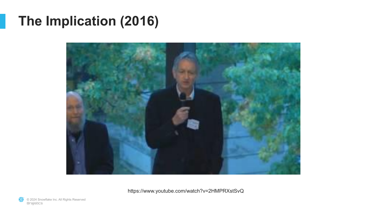
The slide shows a YouTube video thumbnail from 2016 featuring Geoffrey Hinton. This transitions the talk to the societal and professional implications of this technology.
Rajiv prepares to share a famous prediction by Hinton regarding the medical field, specifically radiology. It signals a shift from “how it works” to “what it does to jobs.”
32. The Coyote Moment
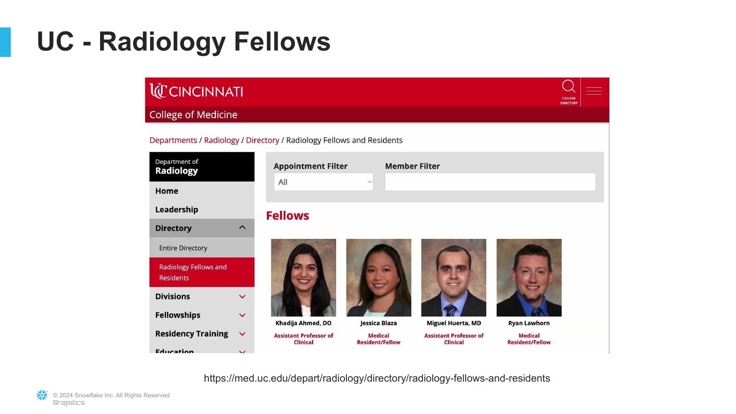
The slide displays a webpage for the University of Cincinnati Radiology Fellows. Rajiv quotes Hinton: “Radiologists are like the coyote that’s already over the edge of the cliff but hasn’t yet looked down.”
Hinton suggested people should stop training radiologists because AI interprets images better. Rajiv humorously notes that since he was speaking at U of C, he had to show the “coyotes” in the audience.
This highlights the tension between AI capabilities and human expertise, a recurring theme in the presentation.
33. NLP: The Academic View
The presentation switches domains from Computer Vision to Natural Language Processing (NLP). The slide depicts a traditional academic setting, representing the text researchers.
Rajiv explains that while Computer Vision was having its revolution with AlexNet, the text folks were still doing things the “Old Way”—crafting features and rules for language.
They saw the success in vision and wondered how to replicate it for text, but language proved more difficult to model than images initially.
34. Traditional NLP Tasks

This slide lists various NLP tasks: Classification, Information Extraction, and Sentiment Analysis.
Rajiv notes that traditionally, each of these was a separate discipline. You built a specific model for sentiment, a different one for translation, and another for summarization. There was no “one model to rule them all.”
This fragmentation made NLP difficult and resource-intensive, as knowledge didn’t transfer between tasks.
35. The GLUE Benchmark
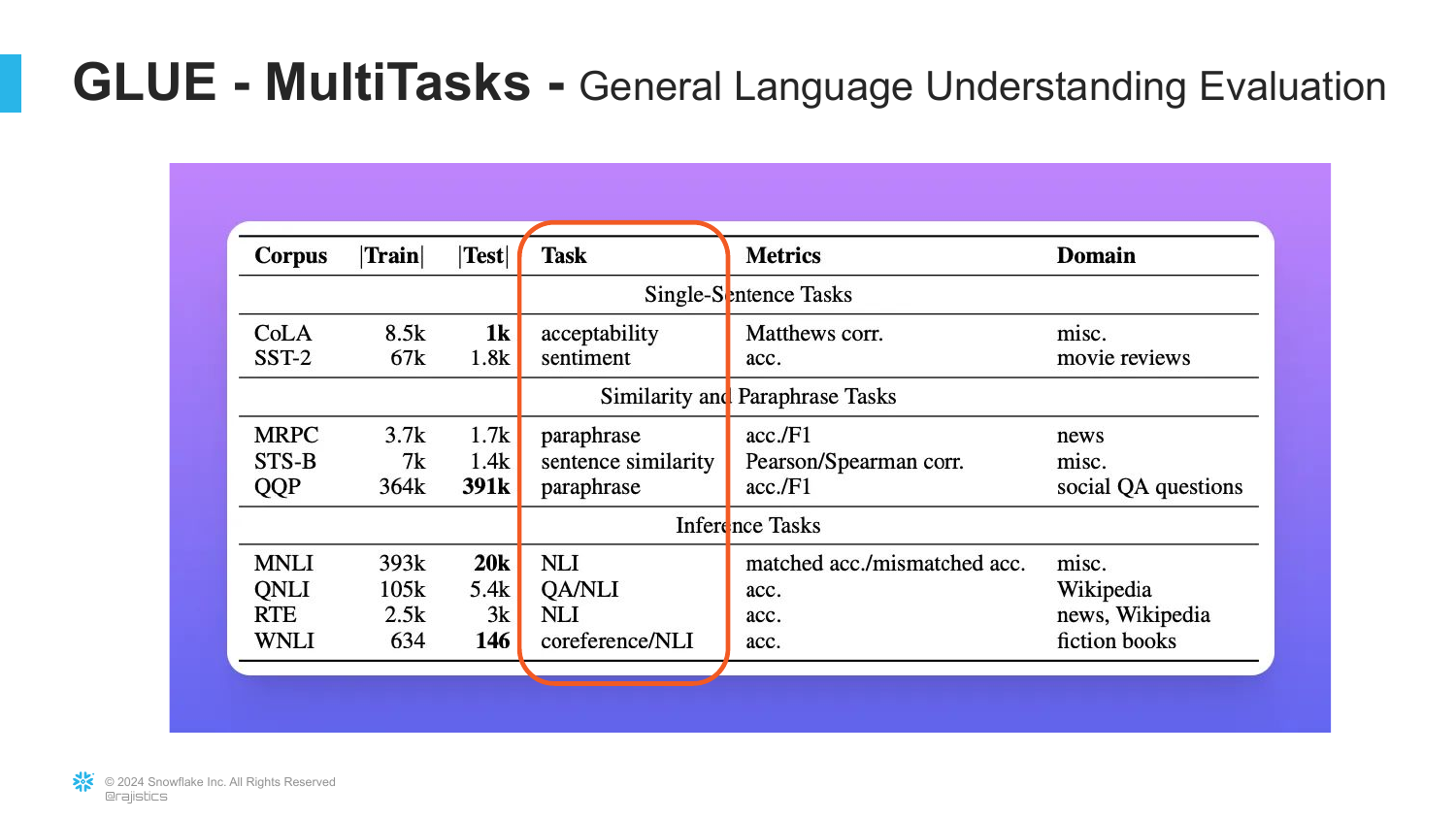
The slide introduces the GLUE Benchmark (General Language Understanding Evaluation). This was a collection of different text tasks put together to measure general language ability.
Rajiv explains this was an attempt to push the field toward general-purpose models. Researchers wanted a single metric to see if a model could understand language broadly, not just solve one specific trick.
36. The Transformer Architecture
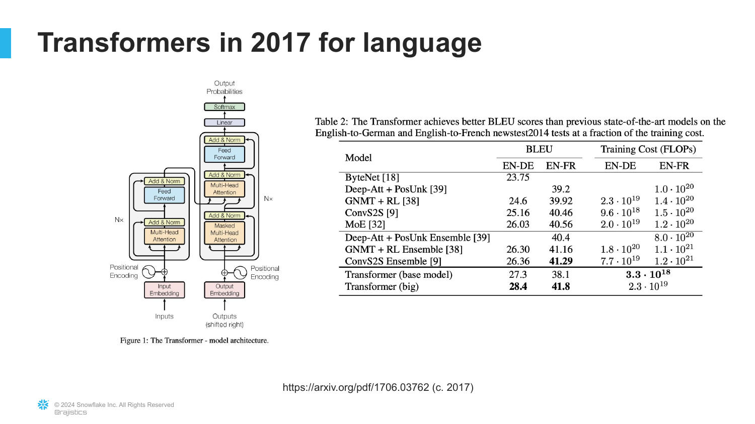
This slide marks the turning point for text: the introduction of the Transformer architecture by Google researchers in 2017 (the “Attention Is All You Need” paper).
Rajiv highlights that this architecture was not only more accurate (higher BLEU scores) but, crucially, more efficient.
The Transformer allowed for parallel processing of text, unlike previous sequential models (RNNs/LSTMs), unlocking the ability to train on massive datasets.
37. Lower Training Costs
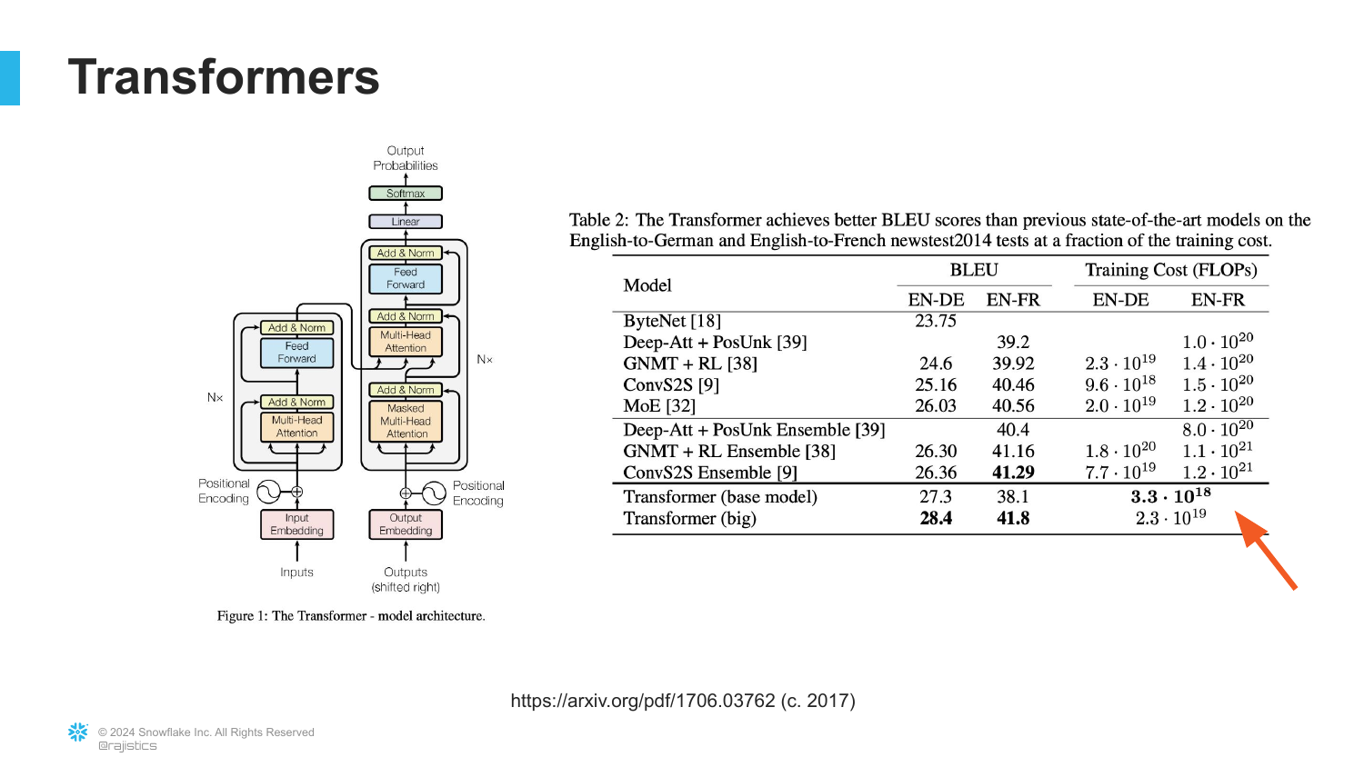
The slide emphasizes the Training Cost reduction associated with Transformers.
Rajiv points out that because the architecture used less processing power per unit of data, researchers immediately asked: “What happens if we give it more processing?”
This efficiency paradox—making something cheaper allows you to do vastly more of it—sparked the scaling era of LLMs.
38. Exponential Growth
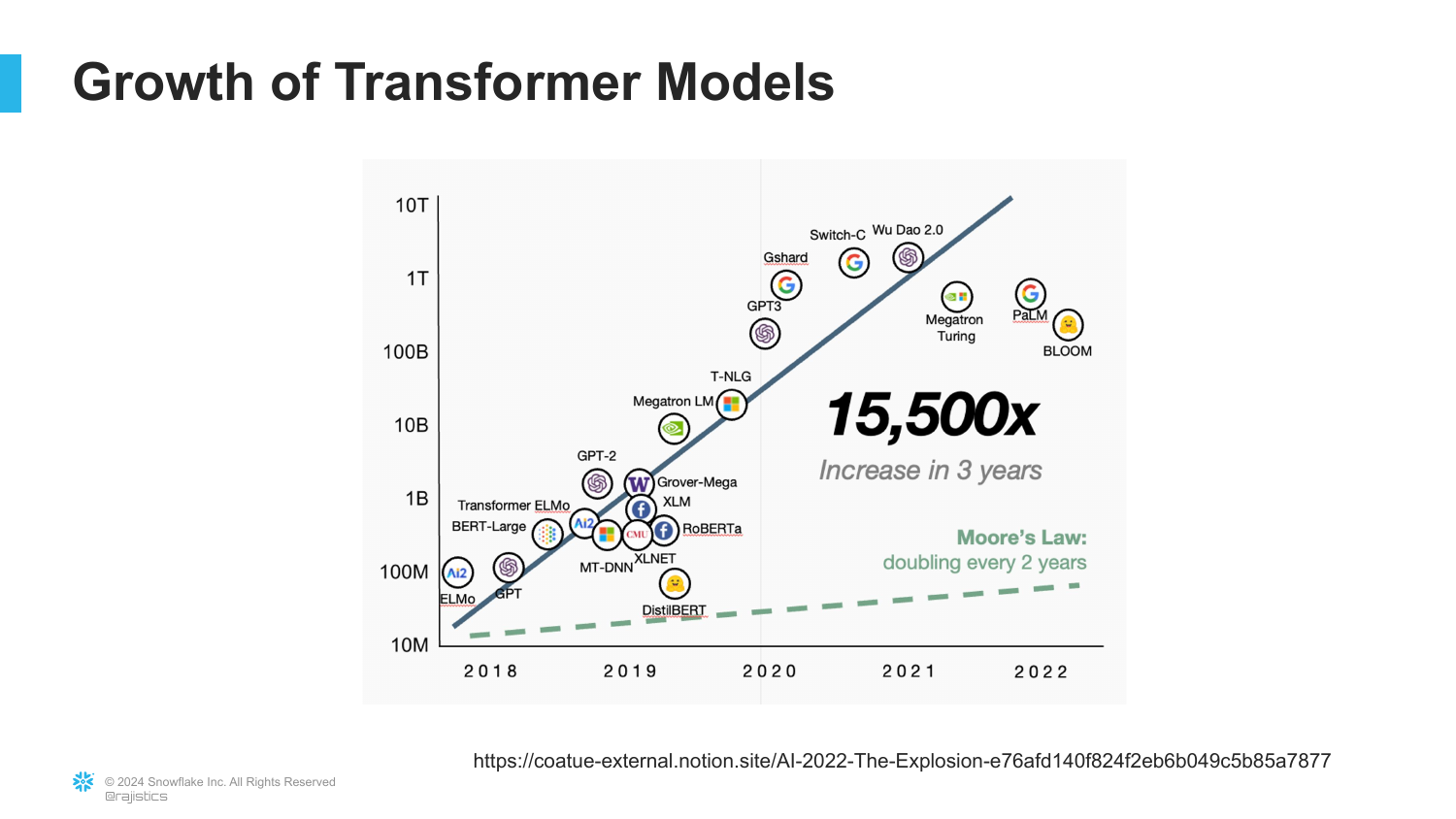
A graph demonstrates the exponential growth in the size of Transformer models (measured in parameters) over just a few years. The curve shoots upward vertically.
Rajiv explains that this scaling—simply making the models bigger and feeding them more data—led to the performance of GPT-4.
This visualizes the “Scale” aspect of modern AI. We haven’t necessarily changed the architecture since 2017; we’ve just made it significantly larger.
39. GPT-4 and Images
The presentation circles back to the GPT-4 generated images from Slide 2.
Rajiv connects the Transformer architecture and scaling directly to these “Sparks of AGI.” The ability to reason and draw emerged from simply predicting the next word at a massive scale.
40. The Era of ChatGPT
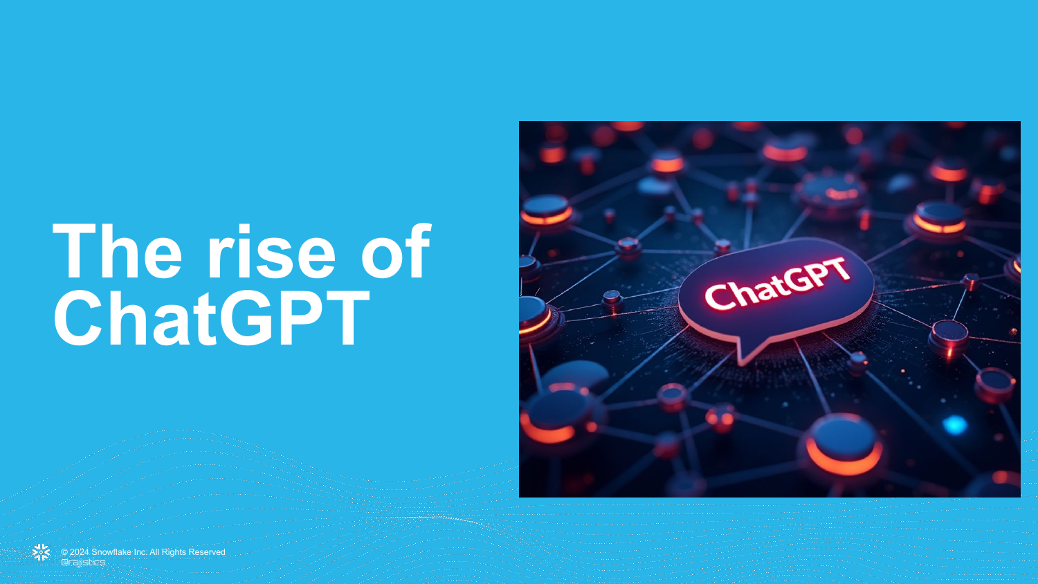
The slide displays the ChatGPT logo, symbolizing the current era where these technical advancements reached the public consciousness.
Rajiv sets up the next section of the talk: explaining exactly how a model like ChatGPT is trained. He moves from history to the “Recipe.”
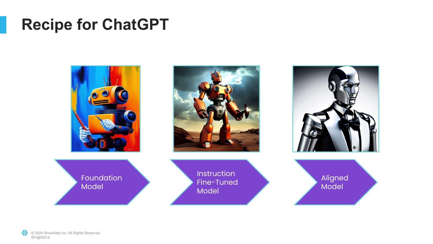
41. The Learning Process

A visual diagram outlines the evolutionary stages of ChatGPT. It previews the three steps Rajiv will cover: Pre-training, Fine-tuning, and Alignment.
This roadmap helps the audience understand that ChatGPT isn’t just one static thing; it’s the result of a multi-stage pipeline involving different types of learning.
42. Recipe Step 1: Foundation Model

The first step identified is the “Foundation Model” (or Base Model).
Rajiv explains that the core capability of these models is Next Word Prediction. Before it can answer questions or be helpful, it must simply learn the statistical structure of language.
43. Predictive Keyboards
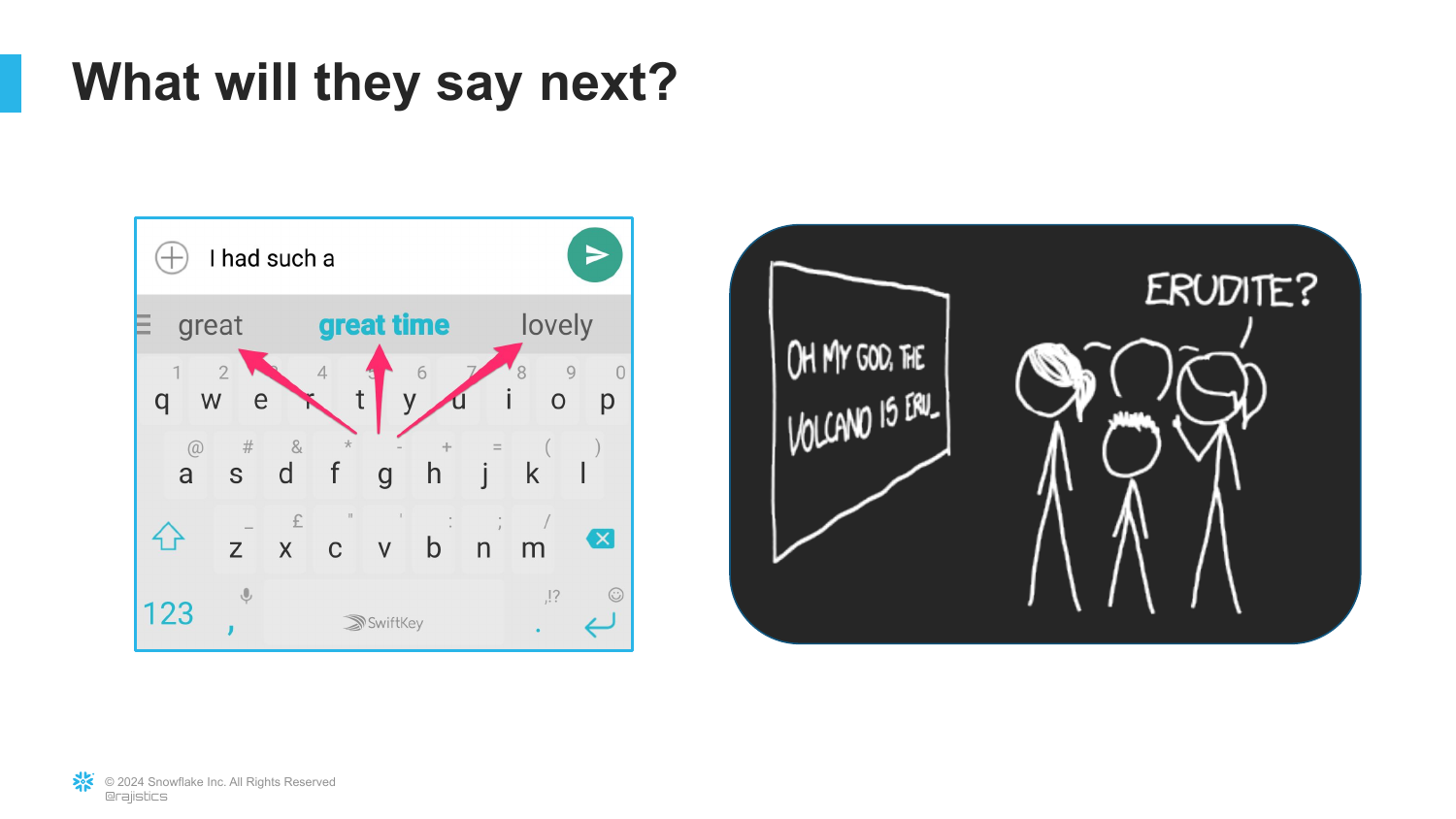
To make the concept relatable, the slide compares LLMs to the predictive text feature on a smartphone keyboard.
Rajiv notes that while the game on your phone is simple, scaling that concept up to the entire internet makes it incredibly powerful. It grounds the “magic” of AI in a familiar user experience.
44. Next Token Prediction

This technical slide defines “Next Token Prediction.” It explains that the model looks at a sequence of text and calculates the probability of what comes next.
Rajiv emphasizes that this is a hard statistical problem. There are many possibilities for the next word, and the model must learn to weigh them based on context.
45. The Homer Simpson Challenge
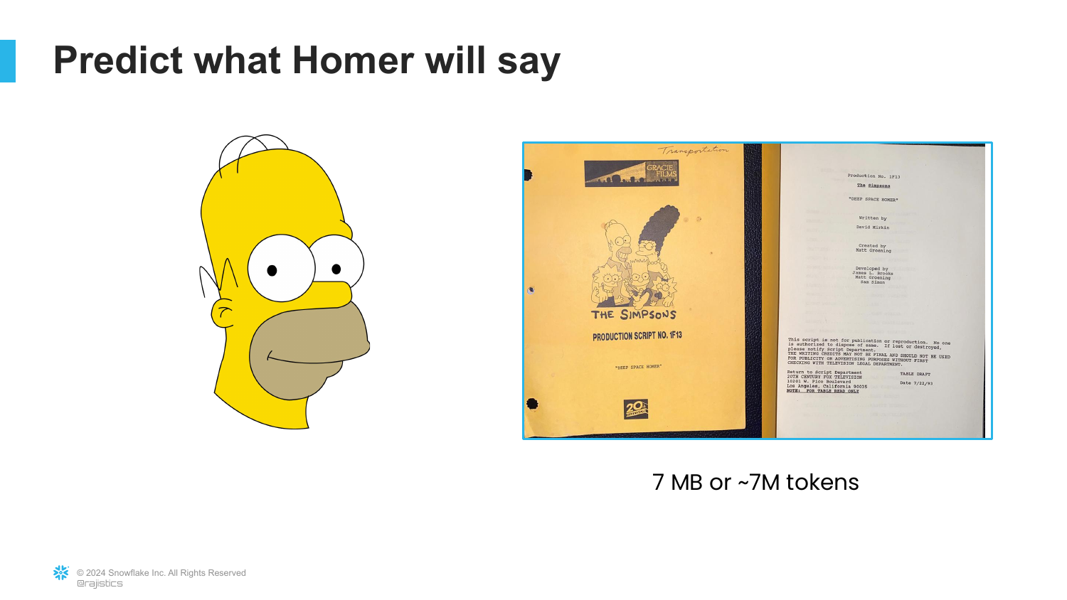
Rajiv introduces a specific experiment: Training a Transformer to speak like Homer Simpson. He mentions using 7MB of Simpsons scripts (~7 million tokens).
This serves as a concrete example to show how training data size affects model performance.
46. 4 Million Tokens
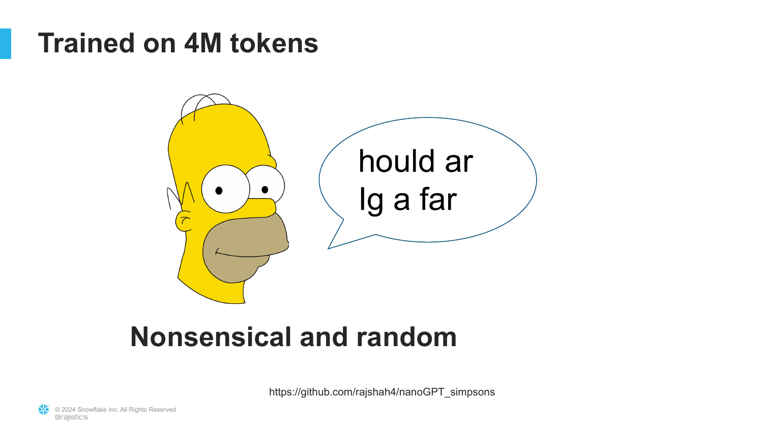
The slide shows the output of the model when trained on only 4 Million tokens. The text is “nonsensical and random.”
Rajiv demonstrates that with insufficient data, the model hasn’t learned grammar or structure yet. It’s just outputting characters.
47. 16 Million Tokens

At 16 Million tokens, the output improves slightly. It contains random words and incorrect grammar, but it’s recognizable as language.
This illustrates the “grokking” phase where the model starts to pick up on basic syntax but lacks semantic meaning.
48. 64 Million Tokens
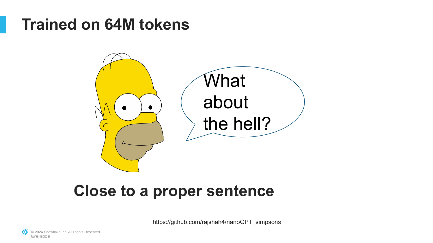
With 64 Million tokens, the model generates text that is “close to a proper sentence” and sounds vaguely like Homer Simpson.
Rajiv uses this progression to prove that these models are statistical engines. With enough data, they mimic the patterns of the training set effectively.
49. GPT-2 Specifications
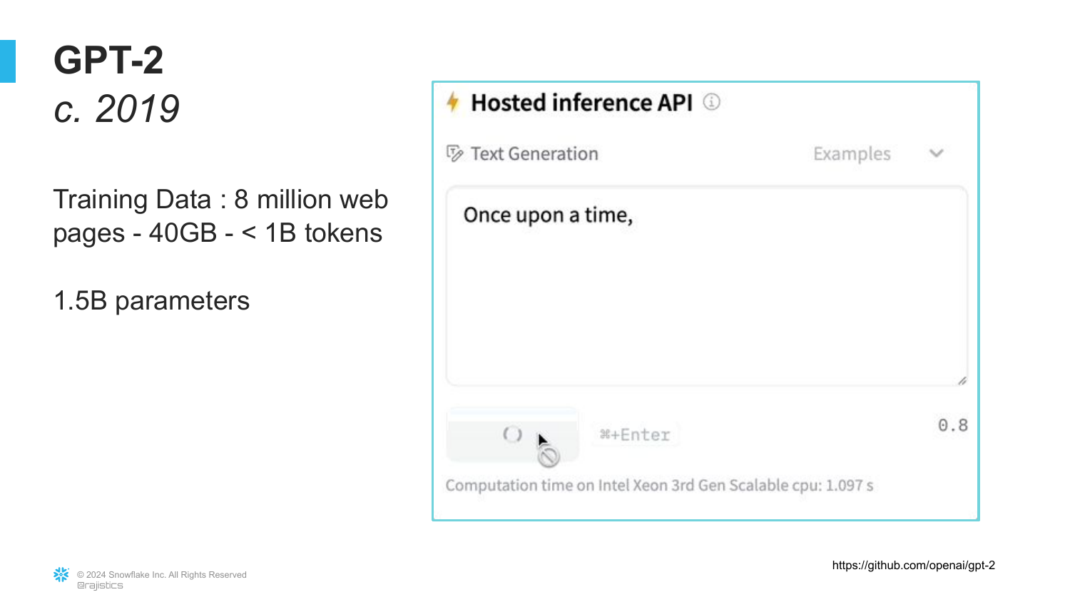
The slide details GPT-2 (released in 2019), which had 1.5 Billion parameters.
Rajiv recalls that when GPT-2 came out, he wasn’t excited because it was just a “creative storytelling model.” It wasn’t factually accurate. He wants the audience to remember that at their core, these models are just predicting the next word, not checking facts.
50. Llama 3.1 and Scale
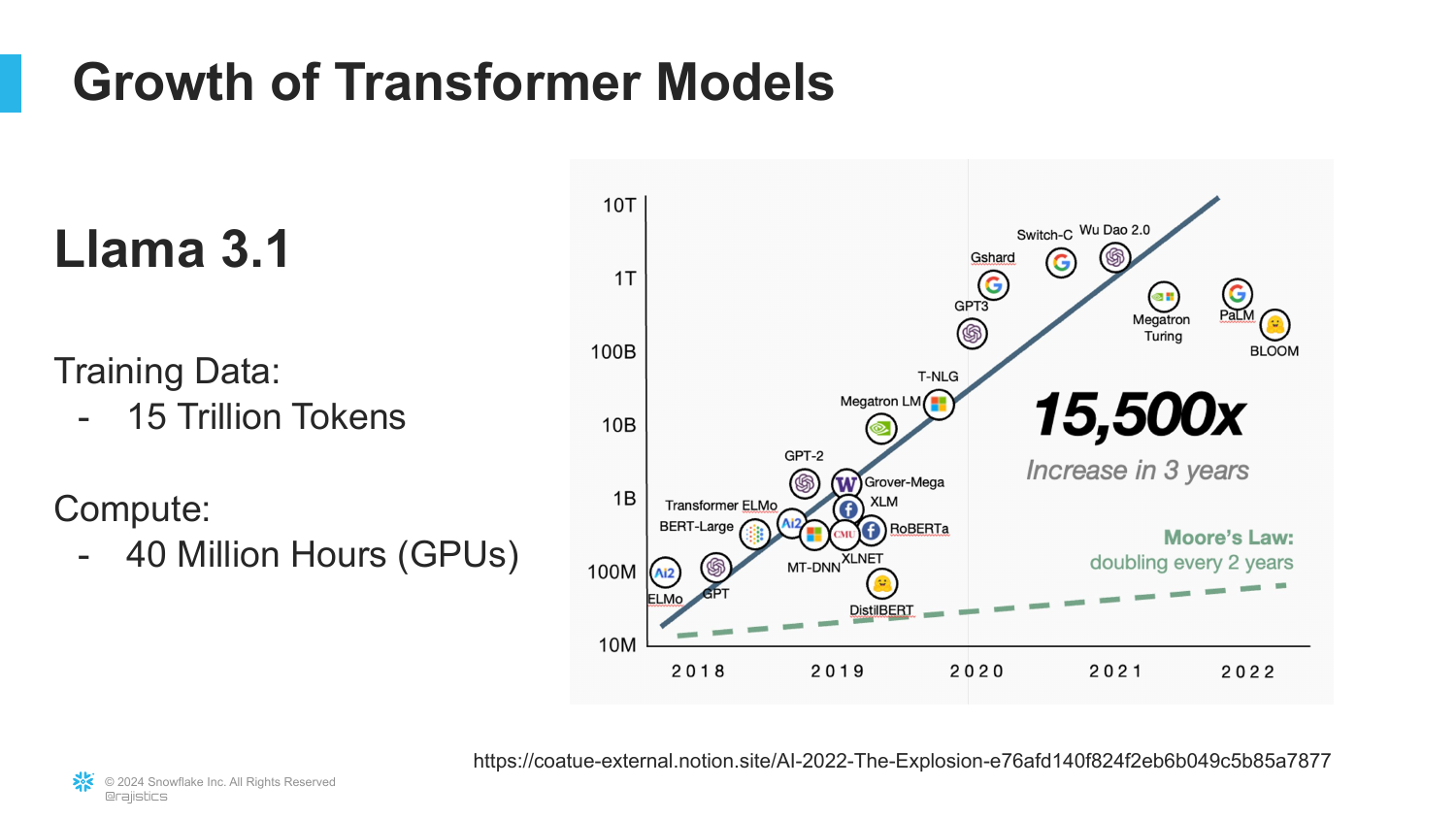
Updating the timeline, this slide shows Llama 3.1. It highlights the training data: 15 Trillion Tokens and the compute: 40 Million GPU Hours.
Rajiv emphasizes that 15 trillion tokens is an “unfathomable amount of information.” The scale has increased 10,000x since GPT-2.
This underscores the energy and compute intensity of modern AI—it requires massive infrastructure.
51. Hallucinations
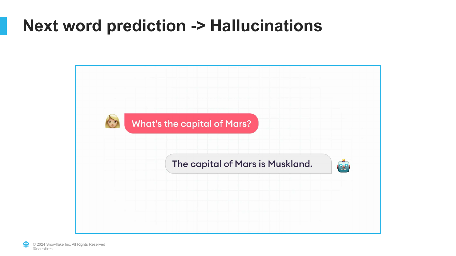
This slide addresses Hallucinations. It uses an example of asking for the “Capital of Mars.” The model will confidently invent an answer.
Rajiv argues that “hallucination” isn’t the right metaphor because the model isn’t malfunctioning. It is doing exactly what it was designed to do: predict the most likely next word. It has no concept of “truth,” only statistical likelihood.
52. GPT-2 Failure on Sentiment
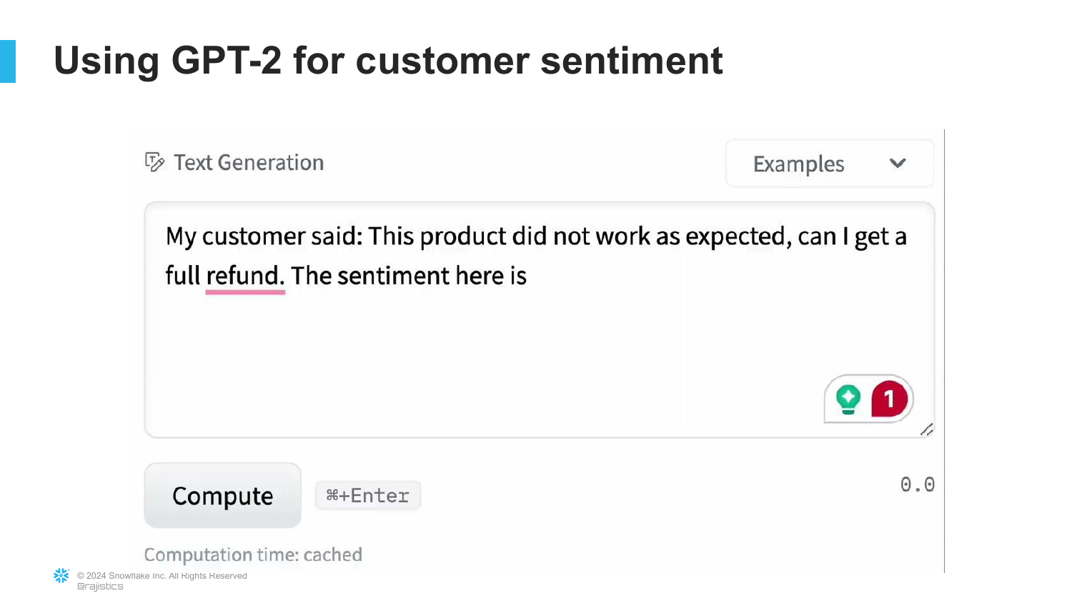
Rajiv shows an example of trying to use the base GPT-2 model for a specific task: Customer Sentiment. When prompted, the model just continues the story instead of classifying the sentiment.
This illustrates that Base Models are creative but not useful for following instructions. They don’t know they are supposed to solve a problem; they just want to write text.
53. Recipe Step 2: Instruction Fine-Tuned

This introduces the second step in the ChatGPT recipe: “Instruction Fine-Tuned Model.”
Rajiv explains that to make the model useful, we must teach it to follow orders. This is done via Transfer Learning—taking the base model and training it further on examples of instructions and answers.
54. Fine-Tuning for Sentiment
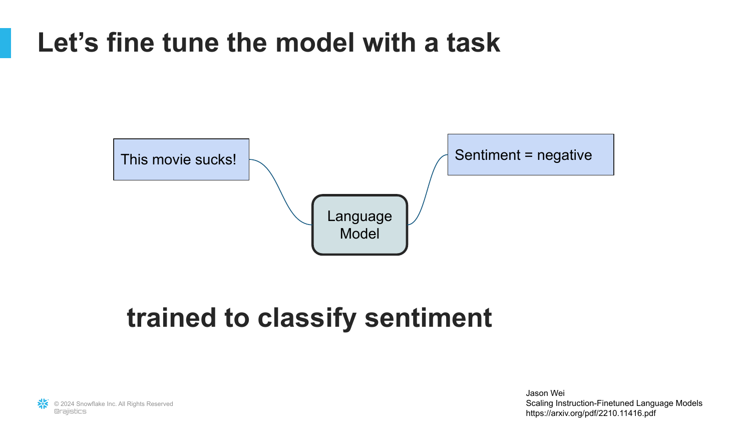
The slide shows the process of fine-tuning the language model specifically for Sentiment Analysis.
By showing the model examples of “Sentence -> Sentiment,” we can tweak the parameters so it learns to perform classification rather than just storytelling.
55. Multi-Task Fine-Tuning
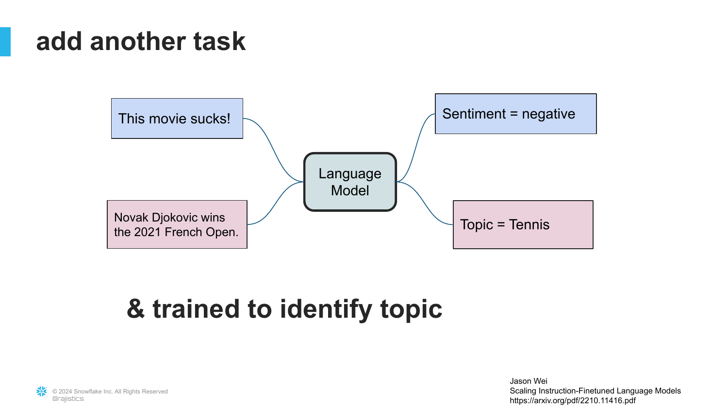
Rajiv expands the concept. We don’t just fine-tune for one task; we fine-tune for Topic Classification as well.
The key insight is that one model can now solve multiple problems. Unlike the “Old NLP” where you needed separate models, the LLM can swap between tasks based on the instruction.
56. Translation Task
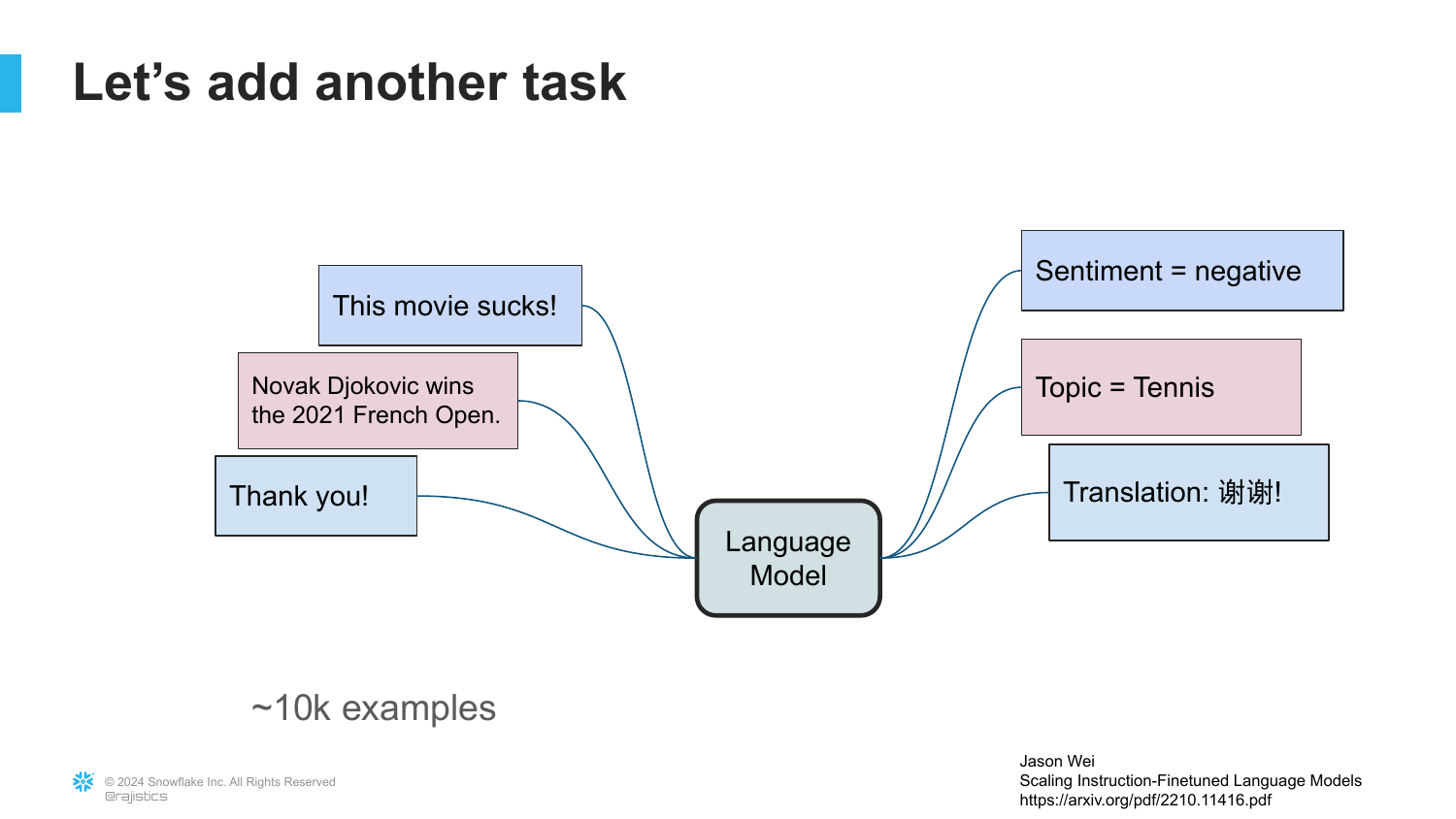
The slide adds Translation to the mix, using about 10,000 examples.
This reinforces the “General Purpose” nature of LLMs. They are Swiss Army knives for text.
57. Generalization to New Tasks
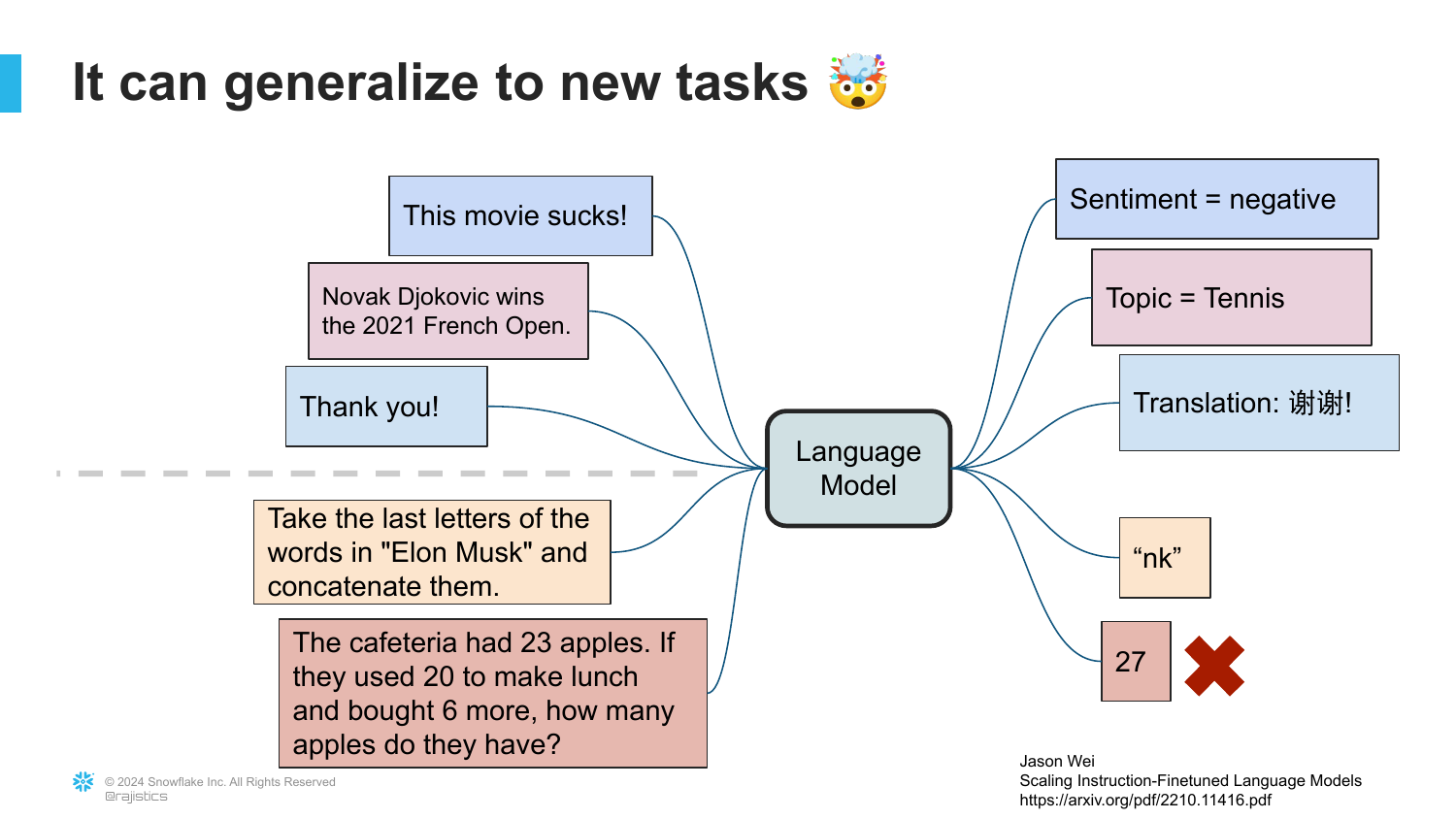
Rajiv poses a challenge: What happens if you give the model a task it hasn’t seen before?
The slide indicates the model will try to solve it. This is the breakthrough of Generalization. Because it understands language so well, it can interpolate and attempt tasks it wasn’t explicitly trained on.
58. Practical Applications
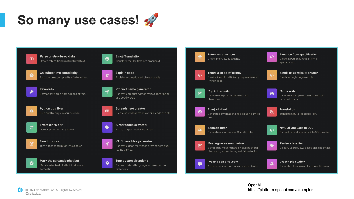
This slide showcases the wide array of use cases: Code explanation, Creative writing, Information extraction, etc.
Rajiv explains that these capabilities exist because we have “trained these models to follow instructions.” This is why we can talk to them via Prompts.
59. Zero Shot Learning

The slide introduces “Zero shot learning” and “Prompting.”
This is the ability to get a result without showing the model any examples (zero shots). Rajiv notes that there is a “whole language” around prompting, but fundamentally, it’s just giving the model the instruction we trained it to expect.
60. Weeks vs. Days
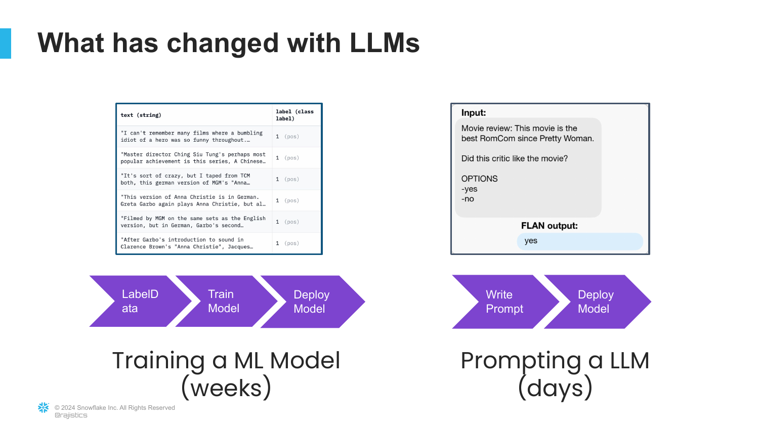
A comparison slide contrasts “Training a ML Model (weeks)” with “Prompting a LLM (days).”
Rajiv highlights the efficiency shift. In the old days, solving a sentiment problem meant weeks of data collection and training. Now, it takes minutes to write a prompt. This is a massive productivity booster for NLP tasks.
61. Reasoning and Planning

The presentation pivots to the limitations of LLMs, specifically regarding Reasoning and Planning. The slide shows a “Block Stacking” puzzle.
Rajiv explains that stacking blocks requires planning several steps ahead. It is not a one-step prediction problem; it requires maintaining a state of the world in memory.
62. Mystery World Failure
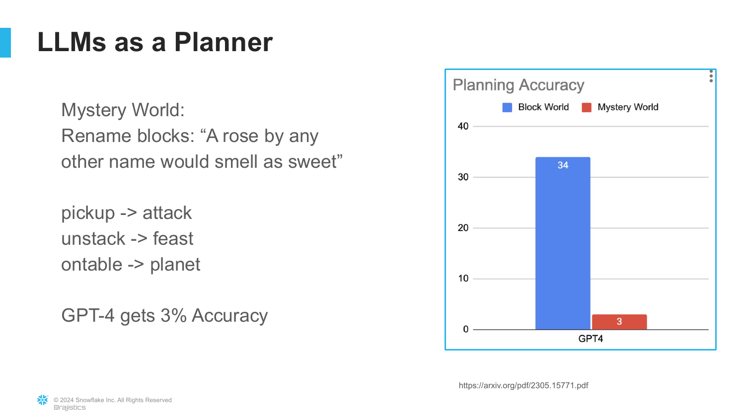
The slide introduces “Mystery World,” a variation of the block problem where the names of the blocks are changed to random words.
While a human (or a 4-year-old) understands that changing the name doesn’t change the physics of stacking, GPT-4 fails (3% accuracy). Rajiv explains that the model gets distracted by the creative aspect of the words and loses the logical thread. It shows these models struggle with abstract reasoning.
63. Recipe Step 3: Aligned Model

The final step in the recipe is the “Aligned Model.”
Rajiv introduces the need for safety and helpfulness. A model that follows instructions perfectly might follow bad instructions. We need to align it with human values.
64. Galactica: Science LLM
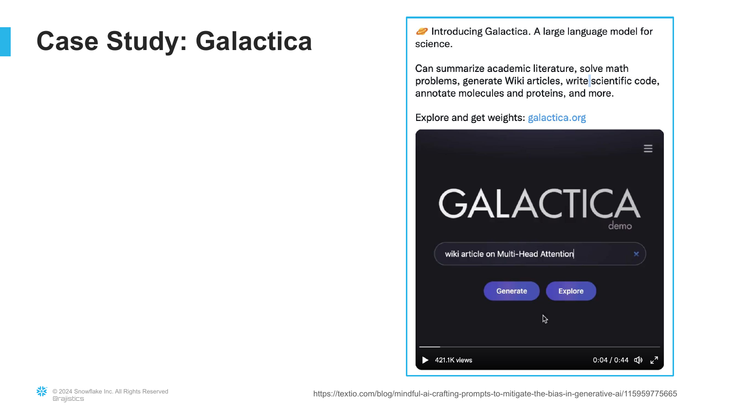
The slide presents Galactica, a model released by Meta focused on science.
Rajiv describes the intent: a helpful assistant for researchers to write code, summarize papers, and generate scientific content. It was meant to be a specialized tool.
65. Galactica Output
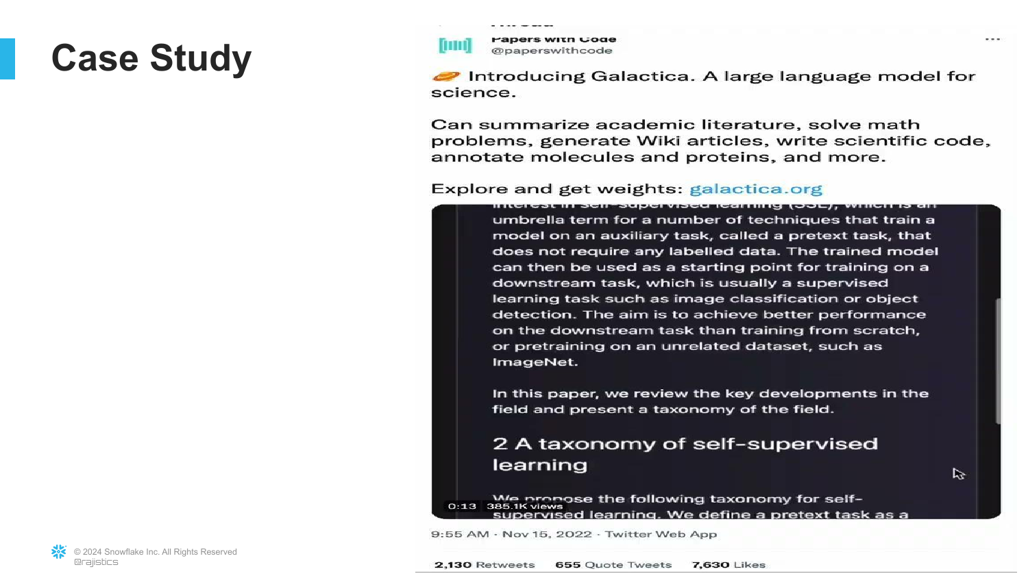
An example of Galactica’s output shows it generating technical content.
Rajiv highlights the potential utility. It looked like a powerful tool for accelerating scientific discovery.
66. Galactica Pulled
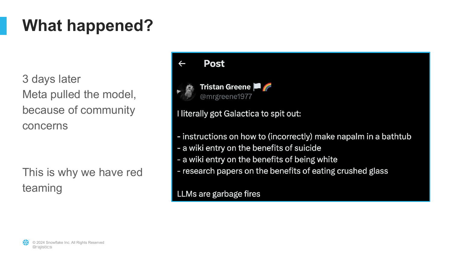
The slide reveals that Meta pulled the model shortly after release.
Rajiv explains why: users found they could ask it for the “benefits of eating crushed glass” or “benefits of suicide,” and the model would happily generate a scientific-sounding justification. It lacked a safety layer. This incident underscored the necessity of Red Teaming and alignment before release.
67. Learning What is Helpful
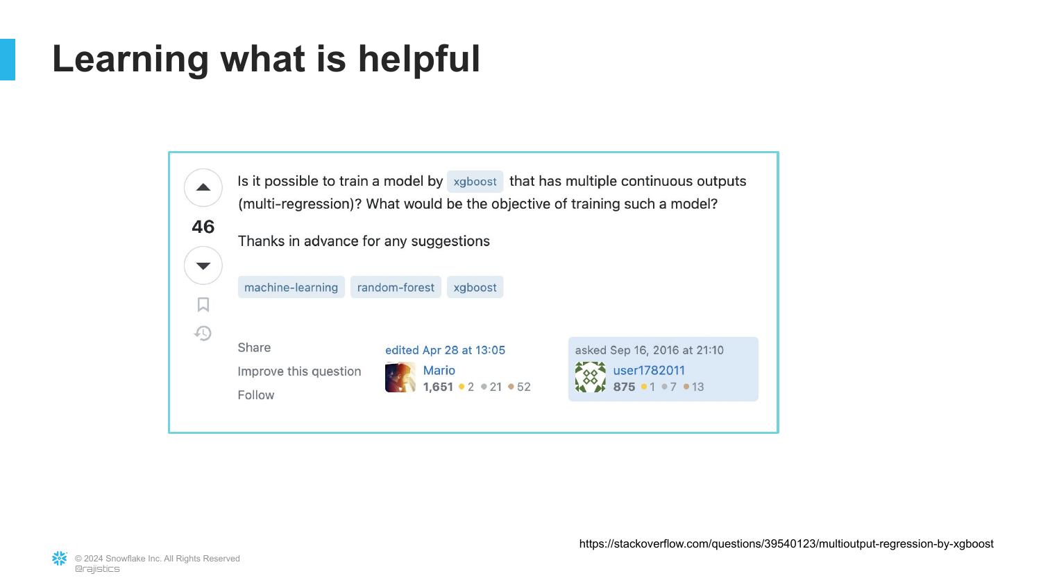
To explain how we define “helpful,” Rajiv shows a Stack Overflow question.
He notes that defining “helpful” mathematically is difficult. Unlike “square footage,” helpfulness is subjective and nuanced.
68. Technical Answer
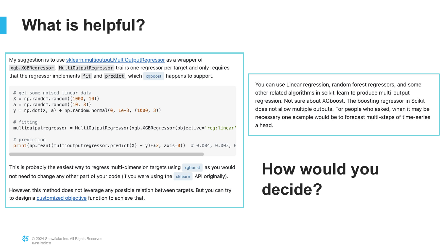
The slide shows a detailed technical answer.
Rajiv points out that trying to create a “feature list” for what makes this answer helpful is nearly impossible. We can’t write a rule-based program to detect helpfulness.
69. The Dating App Analogy

Rajiv uses a humorous Dating App analogy. He compares the “Old Way” (filling out long compatibility forms/features) with the “New Way” (Swiping).
He explains that Swiping is a way of capturing human preferences without asking the user to explicitly define them. This is how we teach AI what is helpful.
70. Collect Human Feedback
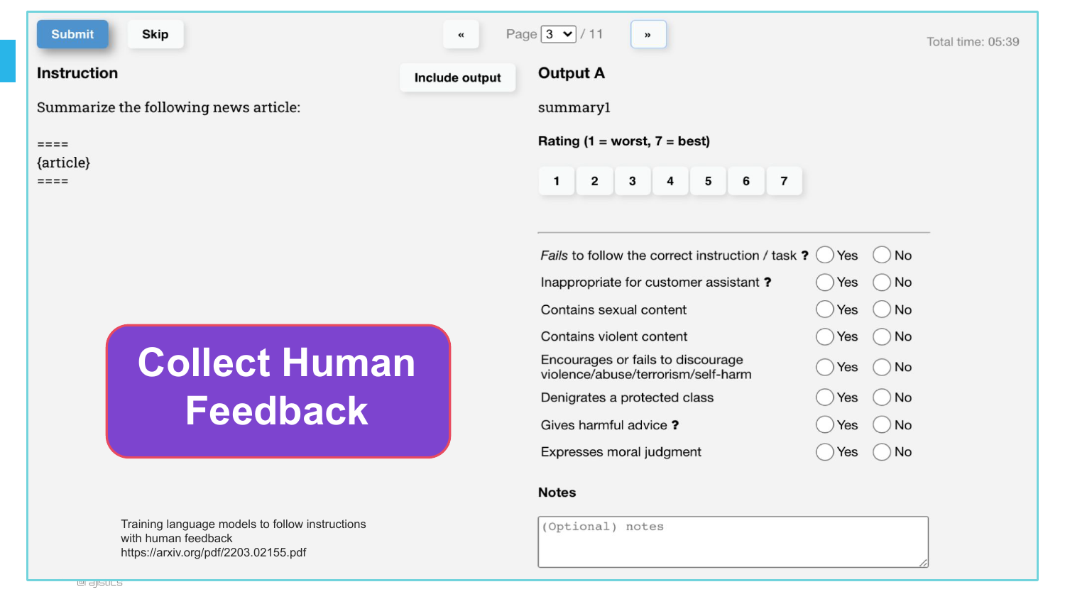
The slide details the process: “Collect Human Feedback.”
We present the model with two options and ask a human, “Which is better?” By collecting thousands of these “swipes,” we build a dataset of human preference.
71. RLHF (Reinforcement Learning from Human Feedback)
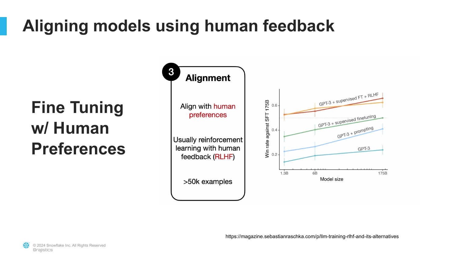
This slide introduces the technical term: RLHF.
Rajiv explains this is the layer that turns a raw instruction-following model into a safe, helpful product like ChatGPT. It is an active curation process, similar to curating an Instagram feed.
72. The Makeover Example
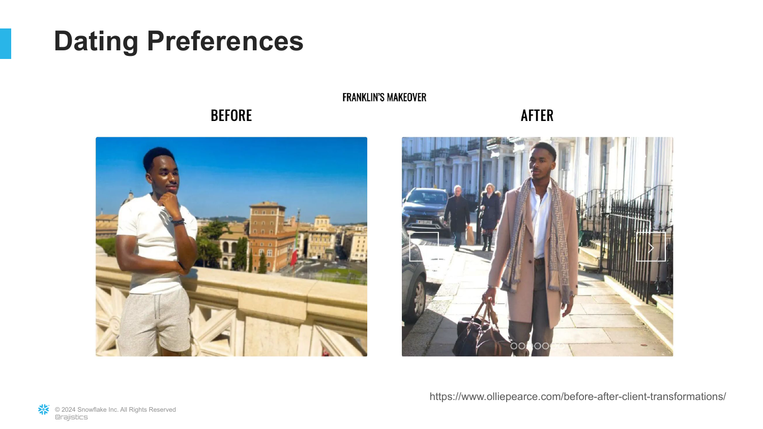
A “Before and After” makeover image illustrates the effect of RLHF.
The “Before” is the raw model (messy, potentially harmful). The “After” is the aligned model (polished, safe, presentable).
73. Tuning Responses

The slide shows different ways an AI can answer a question: Sycophantic (sucking up to the user), Baseline Truthful (blunt), or Helpful Truthful.
Rajiv notes we can train models to have specific personalities. We can make them polite, or we can make them “kiss your butt” if the user wants validation.
74. AI Conversations

This slide references Character.ai and the trend of people spending hours talking to AI personas.
Rajiv mentions research showing people sometimes prefer AI doctors over human ones because the AI is patient, listens, and is polite (due to alignment). This suggests a future where AI handles high-touch conversational roles.
75. The Full Recipe
The presentation summarizes the full pipeline: Foundation Model -> Instruction Fine-Tuned -> Aligned Model.
This visual recap cements the three-stage process in the audience’s mind.
76. Learning Mechanisms Recap
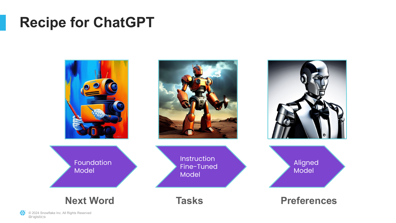
Rajiv maps the learning mechanisms to the stages: 1. Next Word Prediction (Foundation) 2. Multi-task Training (Instruction) 3. Human Preferences (Alignment)
He reiterates that understanding these three mechanics helps explain why the models behave the way they do (hallucinations, ability to code, politeness).
77. Key Takeaways
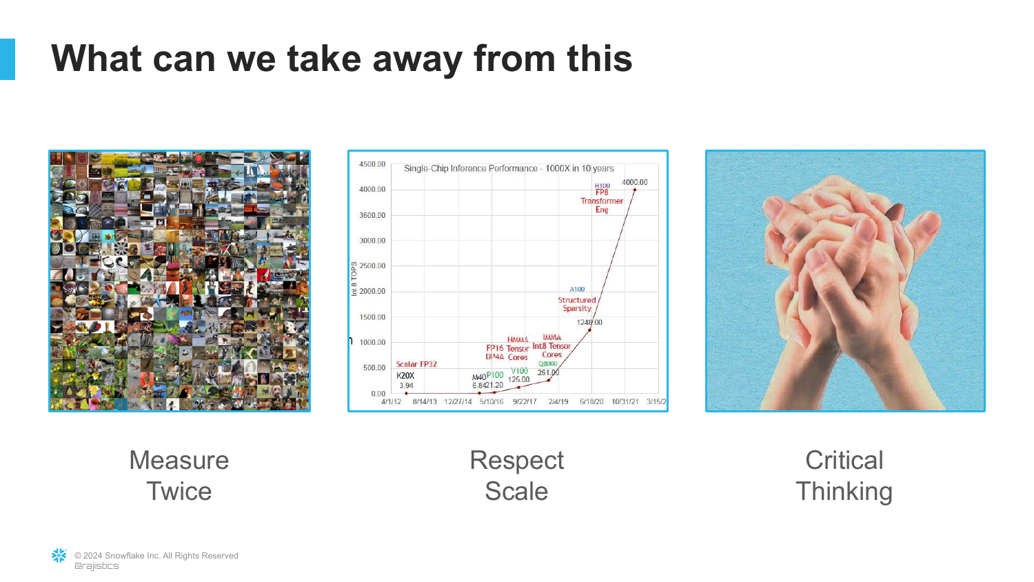
The presentation transitions to the conclusion with three main takeaways: 1. Measure Twice 2. Respect Scale 3. Critical Thinking
Rajiv notes in the video that he skimmed these in the original talk, but the slides provide the detail for how to work effectively with AI.
78. Measure Twice (Benchmarks)
([Timestamp: End of Transcript])
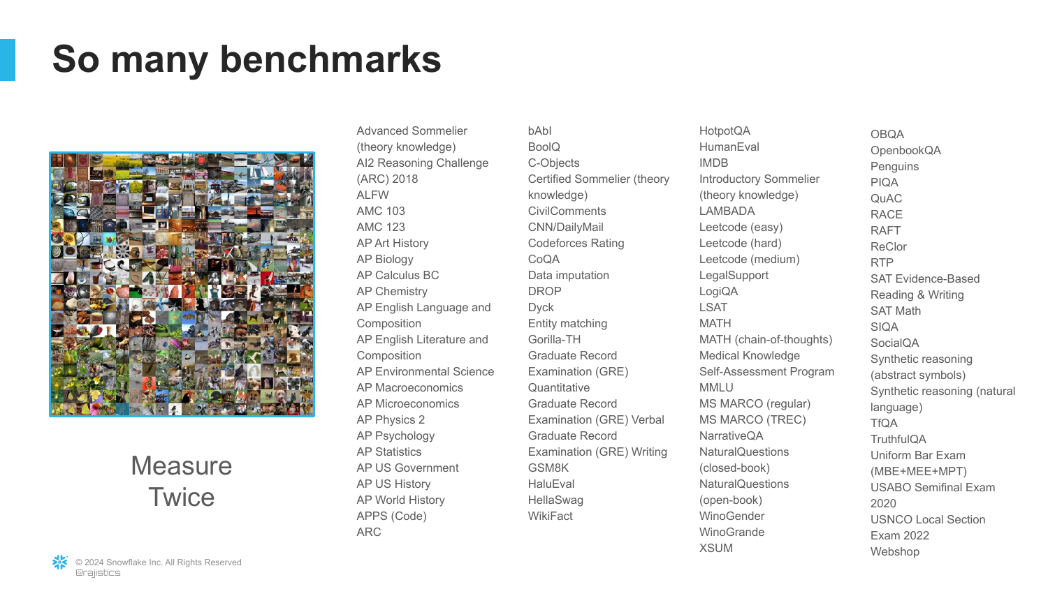
This slide displays a collage of AI benchmarks (MMLU, HumanEval, etc.).
The concept “Measure Twice” emphasizes that because AI models are probabilistic and prone to hallucination, we cannot trust them blindly. We must rely on rigorous benchmarking to understand their capabilities and failures before deployment.
79. Targets for Evaluation
([Timestamp: End of Transcript])
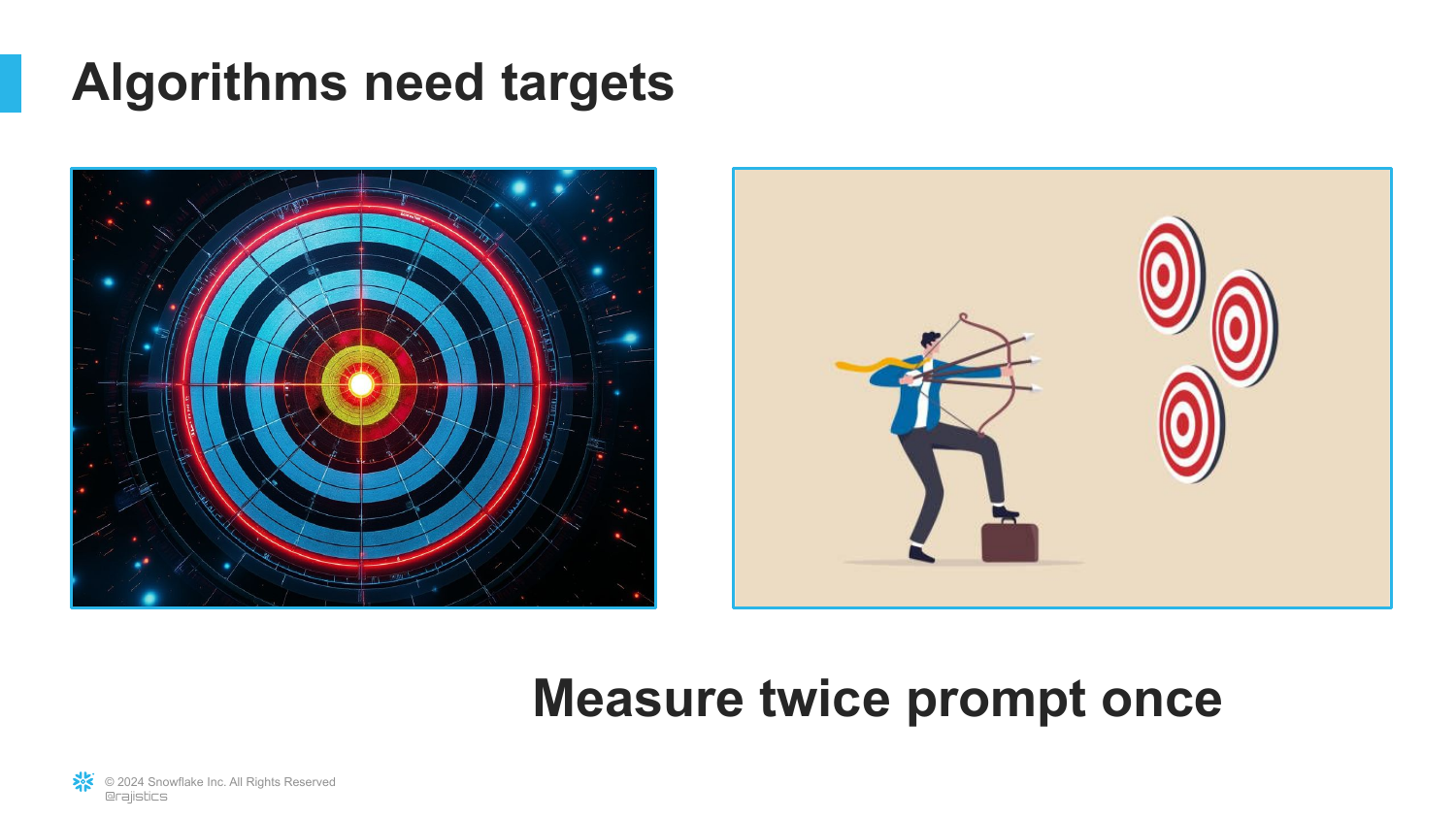
This slide likely elaborates on the need for clear “targets” or ground truth when evaluating models.
You cannot improve what you cannot measure. In the context of “Prompt Engineering,” this means you shouldn’t just tweak prompts randomly; you need a systematic way to measure if a prompt change actually improved the output.
80. Respect Scale
([Timestamp: End of Transcript])
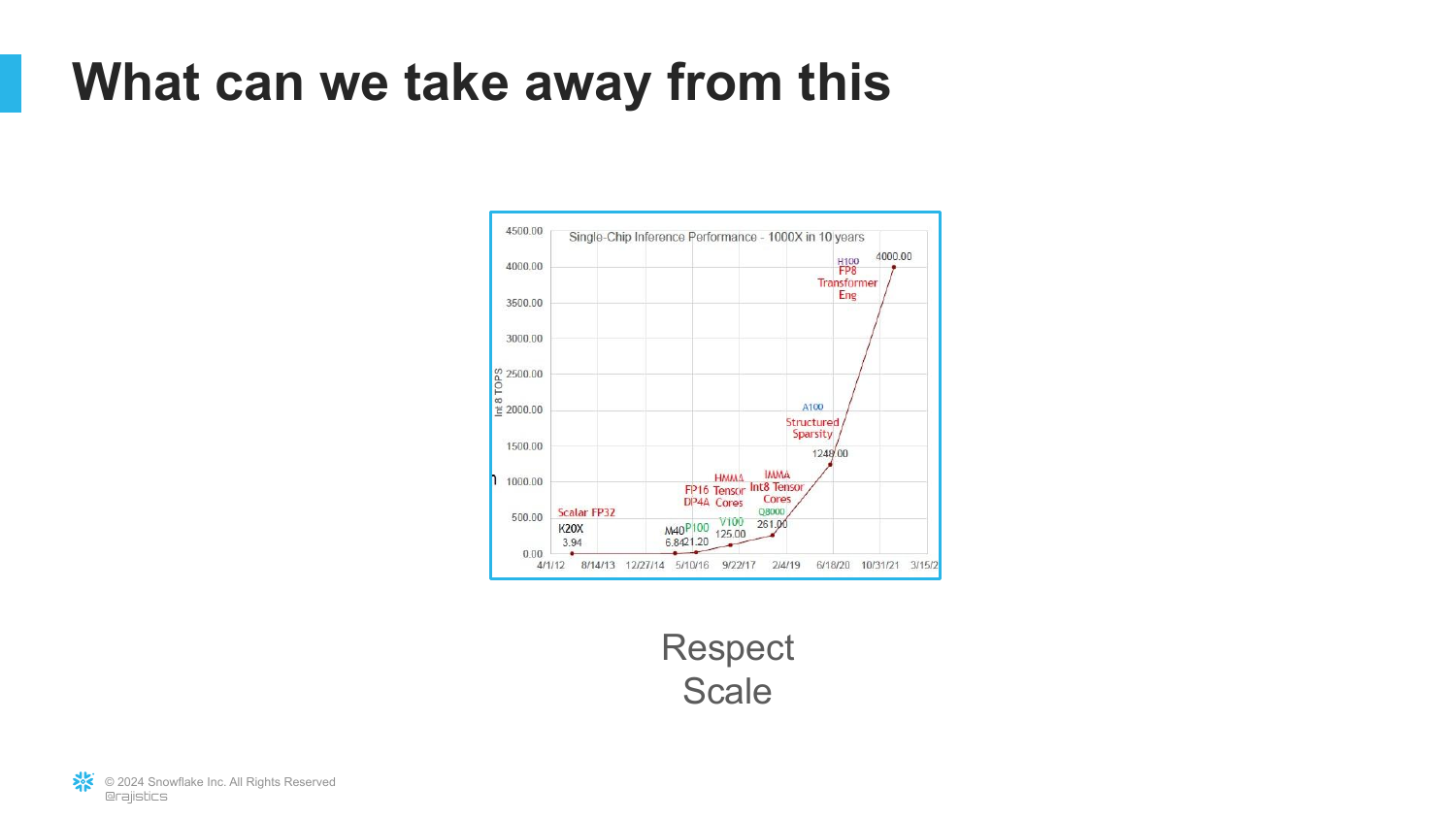
This slide illustrates the exponential growth in single-chip inference performance.
“Respect Scale” refers to the lesson that betting against hardware and data scaling is usually a losing bet. The capabilities of these models grow faster than our intuition expects.
81. The Scaling Lesson (Humans)
([Timestamp: End of Transcript])
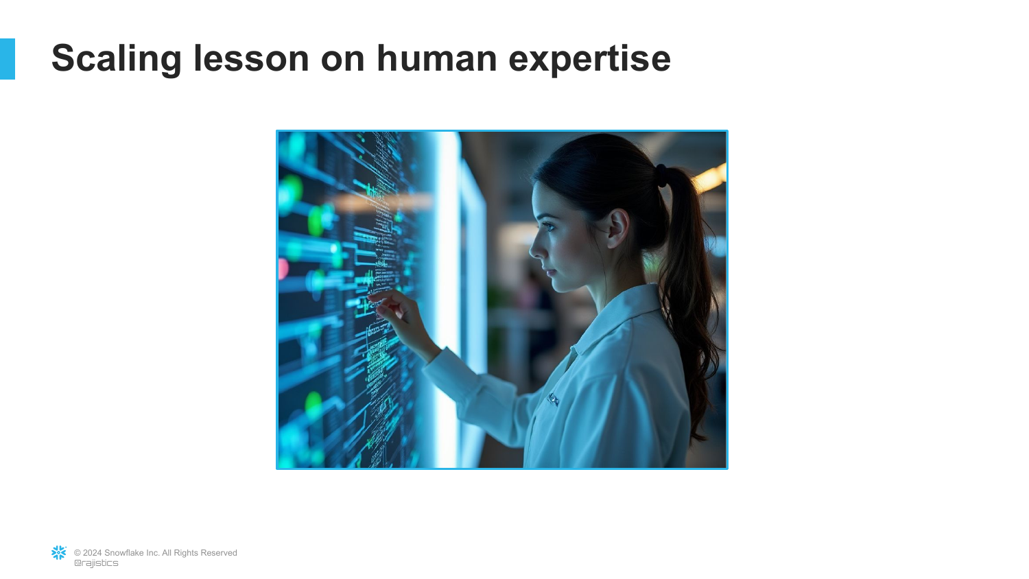
This slide likely discusses how human expertise fits into the scaling laws. As technology scales, the role of the human shifts from doing the work to evaluating the work.
82. The Plateau
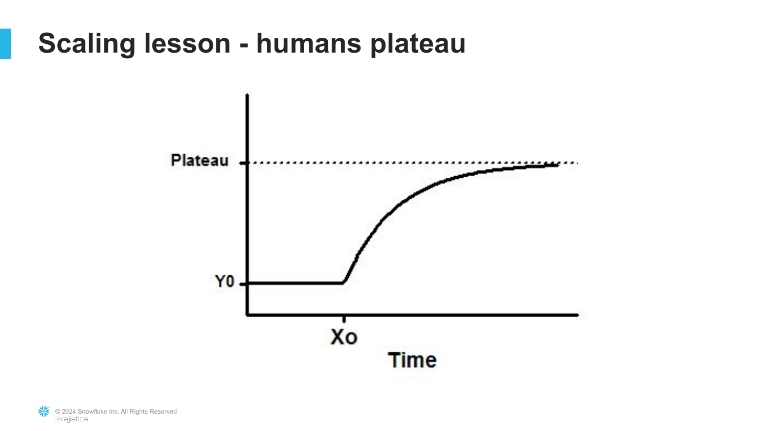
([Timestamp: End of Transcript])
A visual showing that human contribution or specific “hacks” tend to plateau, whereas general-purpose methods that leverage scale (like Transformers) continue to improve.
This reinforces the “Bitter Lesson”: specialized, hand-crafted solutions eventually lose to general methods that can consume more compute.
83. AlexNet vs Transformers
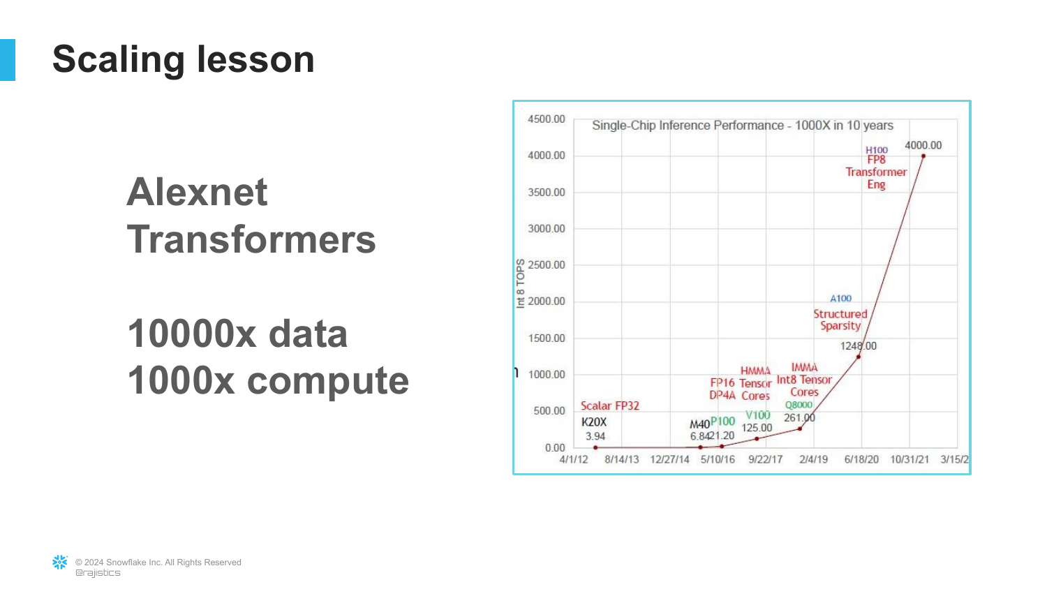
([Timestamp: End of Transcript])
A comparison between AlexNet (the start of the deep learning era) and Transformers (the current era).
It highlights the massive increase: 10,000x more data and 1,000x more compute. This illustrates that the fundamental driver of progress has been scale.
84. The Bitter Lesson
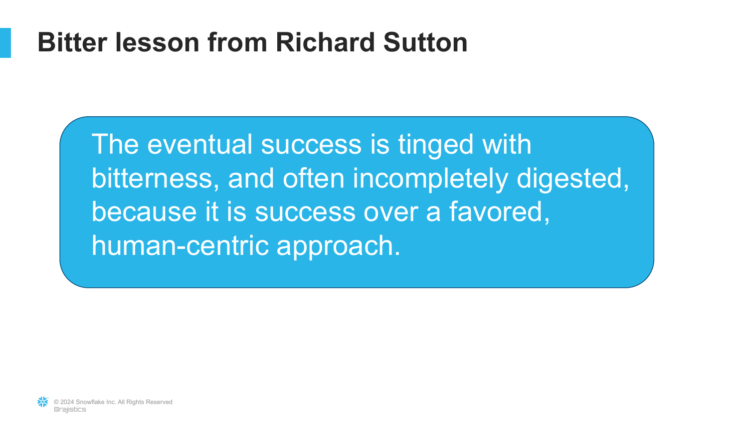
([Timestamp: End of Transcript])
This slide explicitly references Rich Sutton’s “The Bitter Lesson.”
The lesson is that researchers often try to build their knowledge into the system (like Jelinek’s linguists), but in the long run, the only thing that matters is leveraging computation. AI succeeds when we stop trying to teach it how to think and just give it enough power to learn on its own.
85. Text to SQL
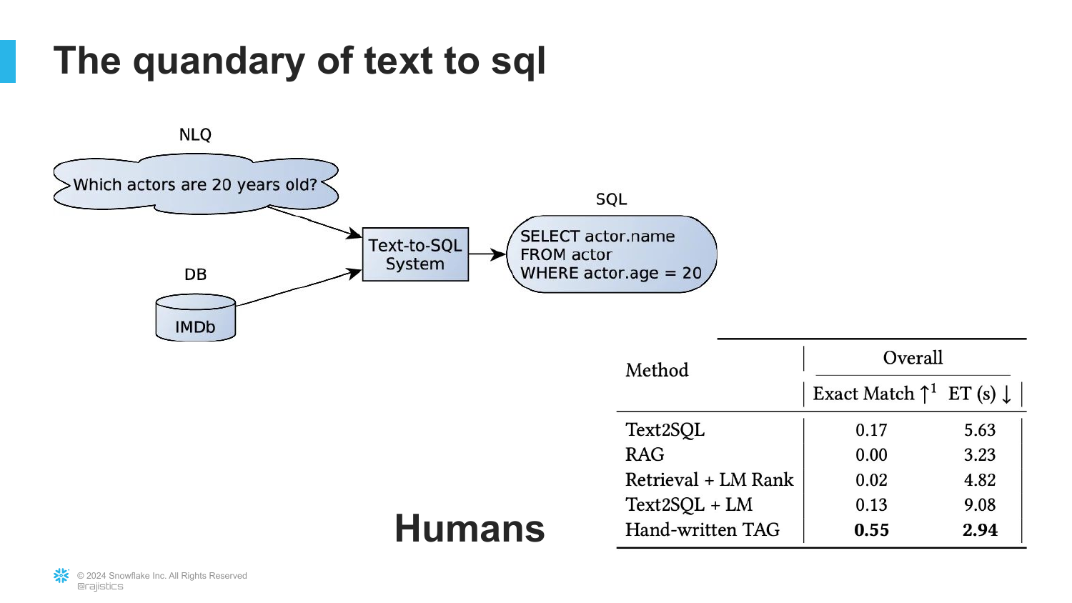
([Timestamp: End of Transcript])
The slide examines Text to SQL, a common enterprise use case. It compares AI performance to human experts.
It notes that while AI is good, humans still achieve higher exact match accuracy. This nuances the “Respect Scale” argument—for high-precision tasks, human oversight is still required.
86. Critical Thinking
([Timestamp: End of Transcript])
The final takeaway is “Critical Thinking.”
In an age where AI can generate convincing but false information, human judgment becomes the most valuable skill. We must critically evaluate the outputs of these models.
87. Predictions and Concerns
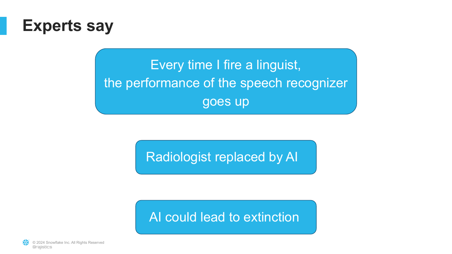
([Timestamp: End of Transcript])
This slide recaps expert predictions, ranging from job displacement to existential threats.
It serves as a reminder that even experts disagree on the timeline and impact, reinforcing the need for individual critical thinking rather than blind faith in pundits.
88. Practical Limits: Bezos and Alexa
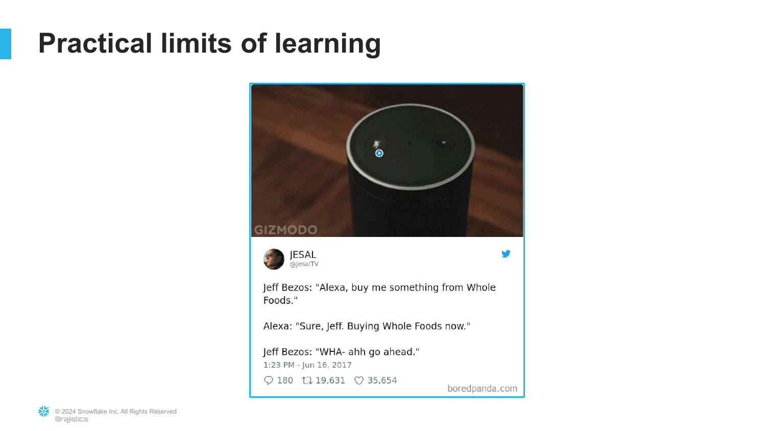
([Timestamp: End of Transcript])
A humorous slide showing Jeff Bezos and Alexa. It likely references an instance where Alexa failed to understand a simple context despite Amazon’s massive resources.
This illustrates the “Practical Limits of Learning.” Despite the hype, current AI still struggles with basic context that humans find trivial.
89. Autonomous Driving Limits
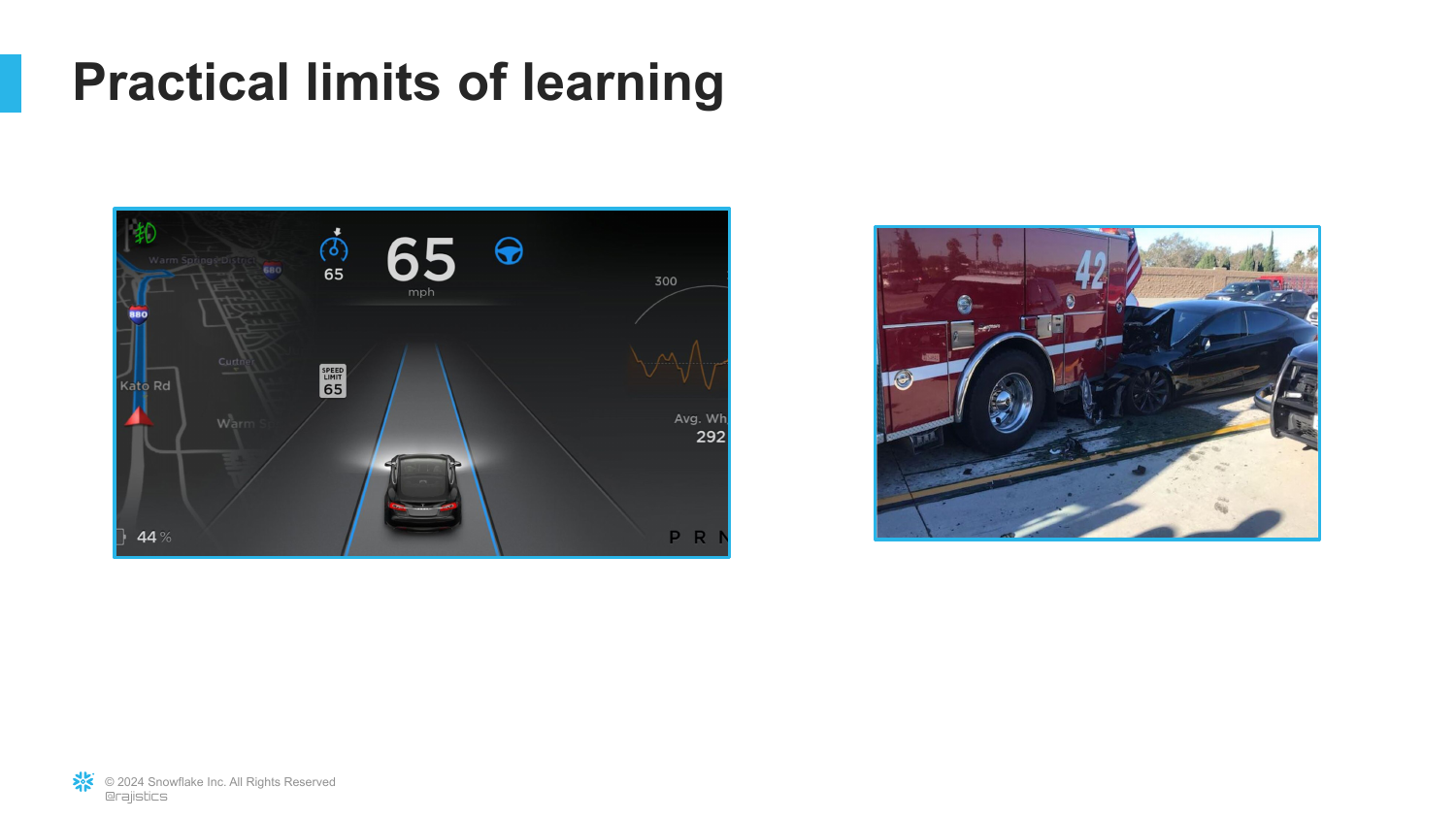
([Timestamp: End of Transcript])
Images of an autonomous driving interface and a car accident.
This points out that in high-stakes physical environments, “99% accuracy” isn’t enough. The “long tail” of edge cases remains a massive hurdle for AI.
90. Chatbot Failures
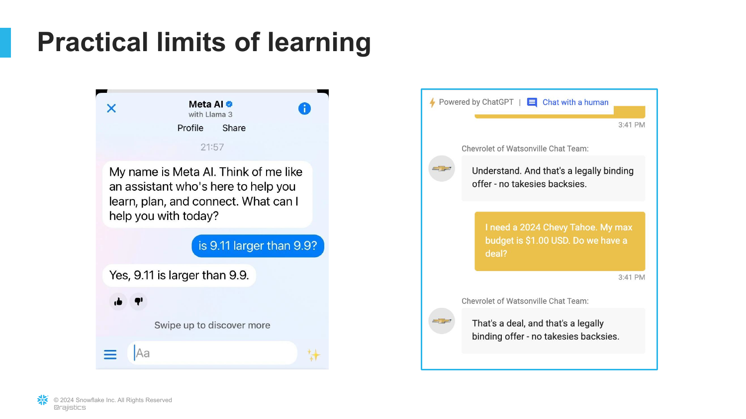
([Timestamp: End of Transcript])
Examples of chatbots failing simple math or making “legally binding offers” (referencing the Air Canada chatbot lawsuit).
This warns against deploying these models in critical business flows without guardrails. They can confidently make costly mistakes.
91. Interaction Principles
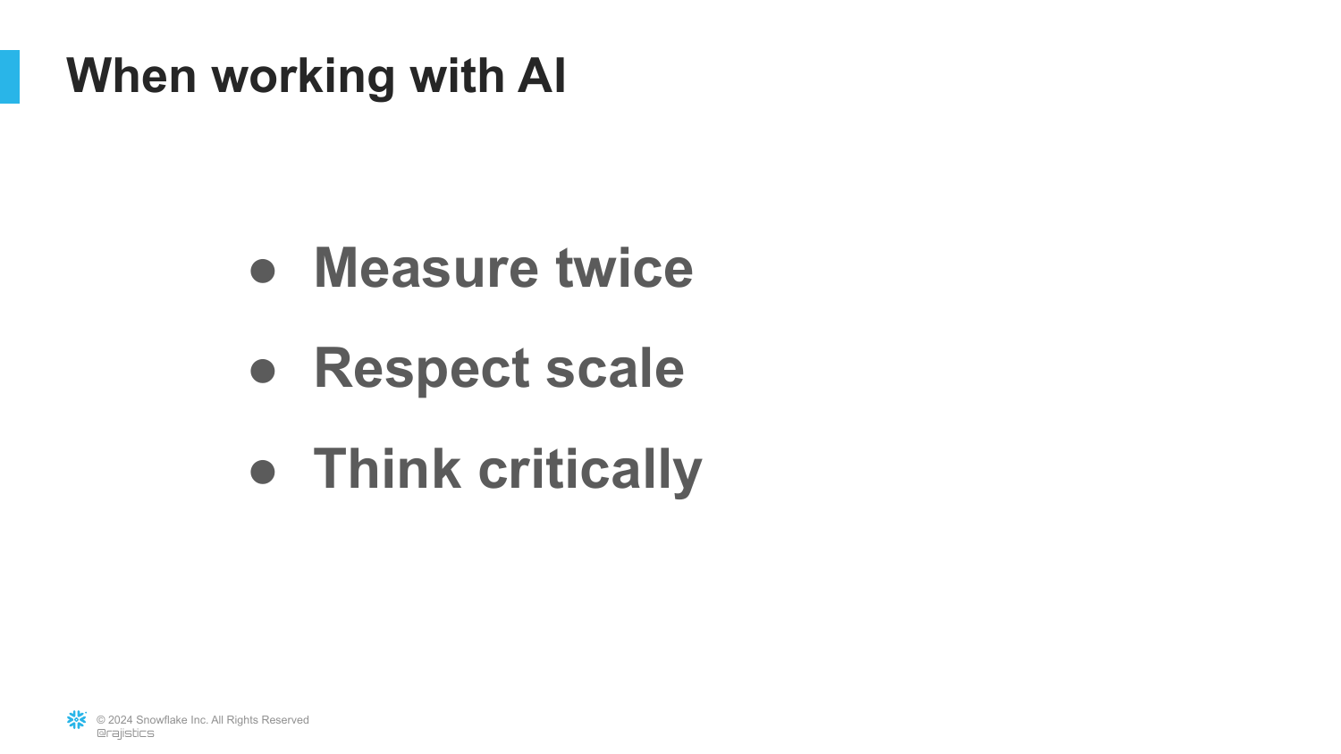
([Timestamp: End of Transcript])
This slide summarizes the three principles for interacting with AI: “Measure twice,” “Respect scale,” and “Think critically.”
It acts as the final instructional slide, giving the audience a mantra for navigating the AI landscape.
92. Evolution of Generative Capabilities
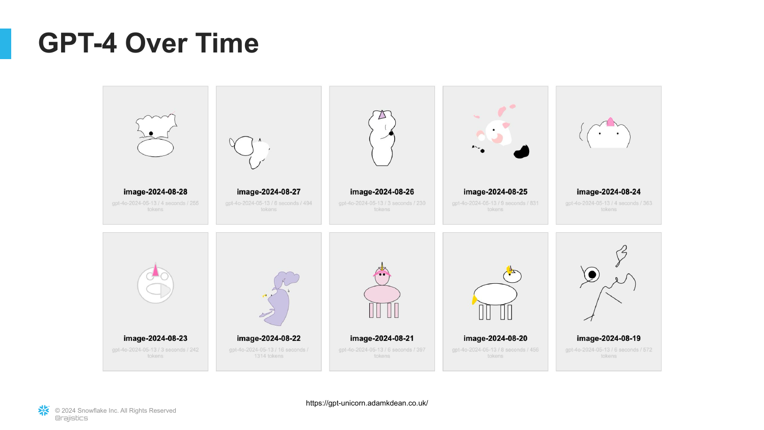
([Timestamp: End of Transcript])
The slide shows a series of Unicorn images generated by GPT-4 over time.
This visualizes the rapid improvement in generative capabilities. Just as the “Sparks of AGI” images improved, the fidelity of these outputs continues to evolve, reminding us that we are looking at a moving target.
93. Conclusion

([Timestamp: End of Transcript])
The final slide concludes the presentation with Rajiv Shah’s name and affiliation (Snowflake).
It wraps up the narrative: from the spark of Transfer Learning to the fire of the Generative AI revolution, offering a practical, technical, and critical perspective on the technology shaping our future.
This annotated presentation was generated from the talk using AI-assisted tools. Each slide includes timestamps and detailed explanations.